Irrigation Engineering 4(3+1)

LESSON 44 Planning and Design of Drip Irrigation System

44.1 Inventory of the Resources and Data Collection

This step involves preparation of inventory of all the available resources and operating conditions. The resources involved include:

Water resources: Quantity (stream size, volume and duration for which the supply is available) and quality of water, the type of water resources i.e. bore/tube well; open dug well, reservoir/pond/tank or river and location of the water resource:

Land resources: The size and shape of the area to be irrigated, soil type for its texture and irrigation properties (field capacity, wilting point, bulk density, allowable depletion level) including infiltration rate, and topography of the land

Climate: The climatic data required for the computation of crop water requirement.

Crop: Crop type, sowing/planting and harvesting period, crop coefficient, fertilser requirements, crop geometry.In general following guidelines can be used to ensure adequate quantity of available water for supply of irrigation water to the wide spaced (orchard) and close spaced (vegetable etc.) crops. However the area to be irrigated can be decided on the basis of the water availability and the crop water demand.

 

Essential parameters		Orchard crops		Vegetables and other closely spaced crops
Stream size		1L s-1/ha-1 for 4hday-1		3Lp-1 ha-1 for 4 h day-1
Storage capacity		15m3ha-1		45m3 ha-1
Power requirement		1hp ha-1		3hp ha-1

 

44.2. Peak Crop Water Requirement

The design of drip irrigation system needs the information on the peak water requirement, however while the system is in operation, the water requirement during the specified irrigation interval is required. This section describes the method to estimate the crop water requirement.Water requirement of crops is a function of plants, surface area covered by plant, evapotranspiration rate. Crop water requirement is calculated for each plant and the water requirement of the whole area is estimated based on the water requirement per plant and total number of plants. The crop water requirement which is maximum during any one of the three seasons is adopted for system design.

 The daily water requirement for fully grown plants can be calculated as under:

                                                                                  (44.1)

Net volume of water to be applied

                                                                                       (44.2)                                            

Number of daily operating hours of the system

                                             (44.3)

                

where,

V  =Volume of water required, L

ET_r= Reference crop evapotranspiration, mm day^-1

_Kc = Crop coefficient

A = Area occupied by a plant (row to row spacing x plant to plant spacing), m²

R_e = Effective rainfall, mm

W_p = Wetting fraction (varies from 0.2 for wide spaced crops and 1.0 for close          spaced crops)

Ne = Number of emitters per plant

N_p = Number of plants

q = Emitter discharge, L h^-1

 

The crop coefficient (Kc) varies with crop growth stage and season. The crop coefficient (Kc) should be considered for the maturity stage of crop while designing micro irrigation system and for the specified growth while operation of the system.

Water requirement of few crops are given in Table 44.1, which can be used as guideline for design of irrigation system. However it should be noted that this is only guideline and actual water requirement needs to be computed on the basis of crop, climate etc.

       Table 44.1.  Water requirements of few horticultural crops

                                                                         

Name of the Crop		Spacing (m)	Water requirement (l/plant/day)
			Minimum	Maximum
Banana		2.0 × 2.0	4	18
Papaya		2.0 × 2.0	2	10
Guava		5.0 × 5.0	14	39
Mango		5.0 × 5.0	20	50
Pineapple		0.45 × 0.25	0.1	0.6
Cashew		7.5 × 7.5	25	60
Jujube		6.0 × 6.0	20	50
Sapheda		5.0 × 5.0	20	65
Pomegranate		5.0 × 5.0	15	40
Tomato		0.6 × 0.6	0.45	1.15
Cauliflower		0.6 × 0.45	0.7	1.4
Okra		0.3 × 0.3	0.6	1.8
Cabbage		0.6 × 0.45	0.7	1.6
Brinjal		0.9 × 0.6	0.8	3.3
Rose		0.75 × 0.75	0.5	2
Jasmine		1.5 × 1.5	1.5	5

 

44.3 Layout of the Drip Irrigation System

It is possible to apply water to the whole field by drip irrigation method at the same time. However this may result in the requirement of high discharge which may not be available, further large diameter of mains and sub main which could make the system more expensive and the high capacities of the fertigation and filtration units. Hence the whole field needs to be divided in to the convenient number of subunits. Each subunit is then designed separately and operated separately by having valve at the head of the subunit. The number of subunits is calculated as:

Number of subunits = Total time available for irrigation/ (time of operation for drip) system (Equation 44.3).

 Total time available for irrigation depends on the hours of electricity available in the region, capacity of the farmers to supplement the electricity by other means such as diesel engine/generator etc.

 The system requirement or discharge for the individual sub unit is then computed. If it is more than the available discharge from the water resources, the area under each subunit is then proportionally reduced to match the discharge requirement with the available discharge,

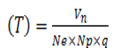
The layout of the micro irrigation system i.e. arrangement of main, sub mains and laterals is done considering the shape, size and slope of the field. As for as possible, the sub main should run along the slope of the field and lateral should be laid across the slope or along the contour lines of the field. Different layouts design of drip irrigation system are shown in Fig. 44.1.

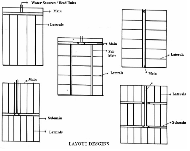
Fig. 44.1. Layout Design of Drip Irrigation System.

(Source: Tiwari, 2009)

 

Once the layout is finalized, the diameter and the length of sub main and laterals for each subunit are decided on the basis of hydraulic design of the pipe which is explained in subsequent sections. The spacing between lateral depends on the crop geometry for the row crops. For the plantation or orchard crops, the spacing between laterals is equal to the row spacing. However depending on the age of tree, tree spacing and soil type, the two laterals per row of tree may be needed. The spacing between the emitters on laterals for row crops is governed by the soil type whereas in case of plantation or tree crops, the number of emitters per tree is governed by the spacing, age and soil type.

44.4 Selection of Emitters

The emitters are to be selected for its discharge, operating pressure, online/inline, pressure compensating/non pressure compensating, point source/line source, single exit/multi exit and surface/subsurface. The selection of particular type of emitter

depends on the soil, crop, topography, desired emission uniformity, available discharge and electricity/other sources for operation of the system, water quality, water use efficiency and the cost.

Soil: The discharge of the emitters should be less than the infiltration rate of the soil. Soil type also governs the spacing between emitters. Heavier the soils, more could be the spacing.

Crop: In case of row crops, emitters need to be spaced so as to wet the entire strip of the row. In case of close growing and row crops, inline/integrated emitters are preferred whereas for the plantation/orchards, online emitters are preferable. Single exit emitters are used for row crops while multi exit emitters are suitable for plantation crops.

 

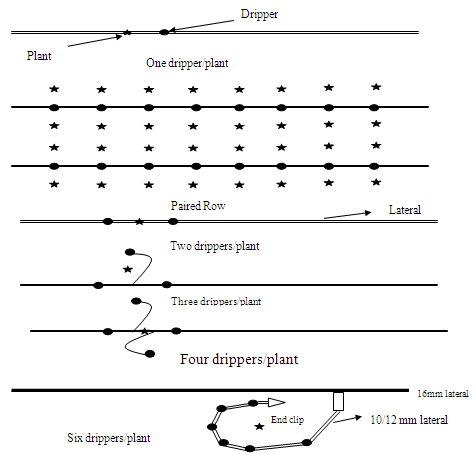
Fig. 44.2. Different arrangement of emitters along the laterals.

 

Topography: Non pressure compensating emitters could be used for relatively flat lands where as on the land with rolling or uneven topography, pressure compensating emitters are preferable.

Emission Uniformity: Pressure compensating emitters are capable of providing more uniformity compared to non pressure compensating emitters.

Discharge Available: When the discharge available is small, the emitters with low discharge need to be used. However these emitters may need more time of operation.

Water Use Efficiency: Subsurface drip irrigation reduces the evaporation losses compared to surface drip; thus resulting in to more water use efficiency

Water Quality: The emitters with more diameter or cross sectional area need to be used for the water with heavy load of suspended solids.

 

44.5 Hydraulic Design of Pipe Network

The pipe network in drip irrigation system consists of laterals, sub main and main. Water under pressure flows through these pipes and as a result the pressure in the pipes reduces creating the variation in pressure or pressure difference between any two points. The emitter discharge depends on the operating pressure available in the pipe at emitter connection and reduces with reducing pressure. Therefore there is variation in discharge obtained by the emitters in system; affecting the emission uniformity.

 Ideally the emitters should give the same discharge at different operating pressure. However only pressure compensating emitters are capable of giving the same discharge over certain range of pressure variation. But these emitters are expensive. The alternative is to design the system with non-pressure compensating emitters such that the same discharge is available at all the points. From the practical point of view, it is almost impossible to achieve this ideal performance. However, the flow variation of water pressure can be minimized by the appropriate hydraulic design.

As per the principle of hydraulics, the minimum pressure variation along the laterals/sub main can be obtained by keeping the diameter of the pipes as large as possible and length as minimum as possible. But doing this is expensive. On the other hand decreasing the diameter and increasing the length, though less expensive, reduces the performance of the system in terms of emission uniformity. In order to have tradeoff between the economy and efficiency, the criterion of allowing the variation in discharge of 10% amongst any two emitters in the subunit is adopted. This is equivalent to 20% variation in pressure for turbulent type of emitters and 10-15% variation for long path emitters. Of the total allowable head loss in the subunit 55% head loss is allowed in laterals and remaining 45% in the sub main.

 

The procedure of hydraulic design consists of:

1.  Know the operating pressure of emitters

2. Find out the allowable head loss in lateral and sub main

3. Find out the lateral and sub main discharge

4. Find out the diameter and length of the lateral such that the head loss in the lateral is within allowable limits for the given layout. For this purpose find out the head loss by Hazen William or Darcy-Wesibach formula for different combinations of diameter and length and select the suitable combination by trial and error method

5. Repeat the procedure for the sub main

6. Find out the diameter of main so that the velocity is within the allowable limit or find out the head loss in main for the specified diameter of the main. The length of the main is the distance of the field from the water source.

 

Computation of Discharge of Lateral, Sub Main and Main

Flow carried by each lateral line

 Q₁ = Discharge of one emitter ´ No. of emitters per lateral

 Flow carried by each sub main line Q =  Q₁ X No. of lateral lines per sub main

 Flow carried by main   Q =  Q₁ X  No. of sub main line

 The diameter of the main, sub main and laterals are chosen based on the hydraulics of pipe flow. The pressure drop due to friction can be evaluated with the help of Hazen William or Dacy-Weishbach equation as stated before.

 

i) Head Loss in Laterals

The pipes used in micro irrigation system are made of plastics (PVC, HDPE, LDPE or LLDPE) and considered as smooth pipe. The pressure drop due to friction or frictional head loss can be evaluated with the help of Hazen -William empirical equation as given below.

              (44.4)           

As the length of the pipe increases, the discharge in the pipe decreases due to emission outlets and hence the total energy drop is less than as estimated by the above equation. For this reason, a reduction factor F which is less than 1.0 is introduced in the equation.

 Head loss for the specified length of pipe is

 Hfl = Hf*(L+Le|)/100

 

where

          H_f (100) = head loss due to friction per 100 meter of pipe length, m/100m

          Hfl = head loss in the specified length of lateral

          Q = Flow of water in pipe, Ls^-1

          D = Internal diameter of pipe, cm

          L = Length of the pipe, m

          C = Hazen-William constant (140 for PVC pipe)

          K = 1.22×10¹²

          Le = equivalent length of the pipe    

= Ne*fe      

Ne = number of emitters on a lateral

fe = equivalent length due to one emitter connection

fe = 1 to 3 m for in line emitter with barbed connection

fe = 0.1 to 0.6 for online emitters

F = Reduction factor due to multiple opening in pipe, which can be computed by following equation.

 

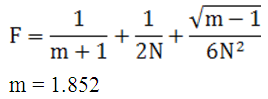
 N = Number of outlets on the lateral

 As stated before, the design criteria for lateral pipe is to keep pressure and discharge variations within the prescribed limit.

 

ii) Head Loss in Sub mains

The sub main line hydraulics of submains pipe is similar to that of the lateral hydraulics.  The sub main hydraulics characteristics can be computed by assuming the laterals are analogous to emitters on lateral line, except for the fact that fe is considered as zero in  this case due to relatively smooth connection of laterals to submain.  Hydraulics characteristics of sub main and mainline pipe for drip system are usually taken hydraulically smooth pipe due to PVC and HDPE pipe material. The Hazen Williams roughness coefficient (C) varies between 140 and 150. The energy loss in the sub main is computed in the same way as used for lateral.

 iii) Head Loss in Main Line

Usually the pressure controls or adjustments are provided at the sub main inlet. Therefore energy loss in the mainline should not affect the system uniformity. In case of main line the value of reduction factor (F) is the unity (1). The frictional head loss in main pipeline is calculated by the same equation Darcy-Weisbach formula or Hazen-Williams.

44.6 Horsepower Requirement of Pump

The horsepower requirement of pump is computed by following equation

 Horsepower required (hp) = 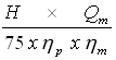                             (44.5)

 

where,

H = total pumping head (H_f + H_e + H_S), m

H_f = Total head loss due to friction (Friction head loss in mains + Friction head loss in sub mains + Friction loss in laterals + Head loss in accessories, filters and fertigation unit), m

H_e = Operating pressure head required at the emitter, m

H_S = Total static head, m

Q_m = Discharge of main                                     

h_p = Efficiency of pump                                    

h_m = Efficiency of motor          

 

References

Tiwari. K. N. (2009). Pressurized Irrigation, Precision Farming Development Center, IIT Kharagpur Publication No. PFDC/ IIT KGP/2/2009: 15.

 

Suggested Readings

Michael, A. M. (2010). Irrigation Theory and Practice, Vikas Publishing House Pvt. Ltd, Delhi, India: 652.

James, Larry G. (1988). Principles of Farm Irrigation System Design, John Wiley and Sons, Inc., New York: 260.