Soil & Water Conservation Structures 3(2+1)

Lesson 5. Peak Rate of Runoff

5.2 Rational Methods

The estimation of peak flow of runoff is particularly important to design various soil and water conservation structures. Rational method is a simple method to estimate peak flow of runoff. In SI units, the equation of rational method that relates the area of watershed (A) in ha, and rainfall intensity (i) in mm/hr(for a duration equal to time of concentration, T_c) with some dimensionless coefficients to peak flow rate (q) in m³/s is given below

                             

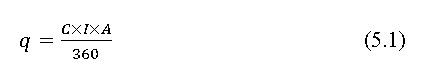
 The runoff coefficient represents the integrated effects of infiltration, evaporation, retention, flow routing and interception, all of which affect peak rate of runoff.

 The runoff coefficient,(C) varies with rainfall rate, land use and cultivation practices, and hydrologic soil groups. The hydrologic soil group B values under different land use are given in Table 5.1. For other hydrologic soil group i.e. A, C and D, there are correction factor which should be multiply to the C values of group B to get the final runoff coefficient. The correction factors are given in Table 5.2.

 Table 5.1: Typical values of runoff coefficient, C for different land use and rainfall intensity for hydrologic soil group B

Crop and Hydrologic conditions	Coefficient C for rainfall rates of
	25 mm/h	100 mm/h	200 mm/h
Row crop, poor practice	0.63	0.65	0.66
Row crop, good practice	0.47	0.56	0.62
Small grain, poor practice	0.38	0.38	0.38
Small grain, good practice	0.18	0.21	0.22
Grassland with rotating species good practice	0.29	0.36	0.39
Permanent pasture under good practices	0.02	0.17	0.23
Forest with matured woodland	0.02	0.1	0.15

(Source: Schwab et al., 1993)

 Table 5.2: Conversion factor to convert runoff coefficient of soil group B to other soil group

Crop and Hydrologic conditions	Conversion factor to convert value of C from soil group B to
	Soil group A	Soil group C	Soil group D
Row crop, poor practice	0.89	1.09	1.12
Row crop, good practice	0.86	1.09	1.14
Small grain, poor practice	0.86	1.11	1.16
Small grain, good practice	0.84	1.11	1.16
Grassland with rotating species good practice	0.81	1.13	1.18
Permanent pasture under good practices	0.64	1.21	1.31
Forest with matured woodland	0.45	1.27	1.40

(Source: Schwab et al. 1993)

 Table 5.3: Runoff coefficient as affected by slope

Hydrologic Soil Group	Slope (%)	Land use/cover
		Forest	Meadows	Pasture	Farmland
A	<2%	0.08	0.14	0.15	0.14
	2-6%	0.11	0.22	0.25	0.18
	>6%	0.14	0.30	0.37	0.22
B	<2%	0.10	0.20	0.23	0.16
	2-6%	0.14	0.28	0.34	0.21
	>6%	0.18	0.37	0.45	0.28
C	<2%	0.12	0.26	0.30	0.20
	2-6%	0.16	0.35	0.42	0.25
	>6%	0.20	0.44	0.52	0.34
D	<2%	0.15	0.30	0.37	0.24
	2-6%	0.20	0.40	0.50	0.29
	>6%	0.25	0.50	0.62	0.41

(Source:http://www.knoxcounty.org/stormwater/pdfs/vol2/313%20Rational%20Method .pdf)

 Rational Formula for Multiple Land Use

The runoff coefficient for composite land use are modified as weighted average over area and is given as

 

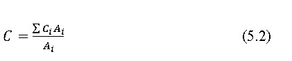
 Where, C_i is the runoff coefficient for i type land use and A_i is the area for the i type land.

 5.3 Time of Concentration

The Rational method uses the rainfall intensity for the duration equal to the time of concentration. The time of concentration is the time lag to reach the generated runoff at remotest point of the watershed to the outlet. The time of concentration is related to the geomorphological characteristics of the watershed such as watershed slope and length of main channel. The following empirical relationship between time of concentration and channel length and slope is given by Kirpich (1940):

 

                   

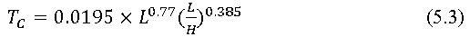
Where, Tc is time of concentration (min), L is length of main channel (m) and H is elevation different between outlet and remotest point in the watershed (m). The T_c thus obtained is used to establish rainfall intensity using intensity-duration-frequency curve.

 5.4 Rainfall Intensity Duration and Frequency (IDF relationship)

The intensity-duration-frequency (IDF) curve is a set of characteristics curve that describe the rainfall characteristics specific to the region. In many design problems related to watershed management, it is necessary to know the rainfall intensities of different durations and different return periods. It takes into the account of probabilistic of the rainfall to exceed certain intensity and its frequency in the selected return period. The inter-relationship among the intensity, i, (mm/h), duration, D (h) and return period, T (years) is described below:

 

                                            

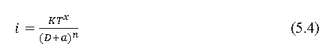
 K, T, a and n are the constants. These constant are specific to the given catchment.

 

(Source:https://www.google.co.in/search?hl=en&site=imghp&tbm=isch&source=hp&biw=1517&bih=740&q=Intensity-duration-frequency+curves&oq=Intensity-durationfrequency+curves&gs_l=img.12..0i24.16551.16551.0.18127.1.1.0.0.0.0.390.390.3-1.1.0....0...1ac.2.32.img..0.1.390.iazYXOvgAE4#facrc=_&imgdii=_&imgrc=DvvBv6gM9pSPM%3A%3BRXfH4uFp24m5dM%3Bhttp%253A%252F%252Fecho2.epfl.ch%252FVICAIRE%252Fmod_1a%252Fchapt_3%252Fpictures%252Ff14.gif%3Bhttp%253A%252F%252Fecho2.epfl.ch%252FVICAIRE%252Fmod_1a%252Fchapt_3%252Fmain.htm%3B383%3B241)

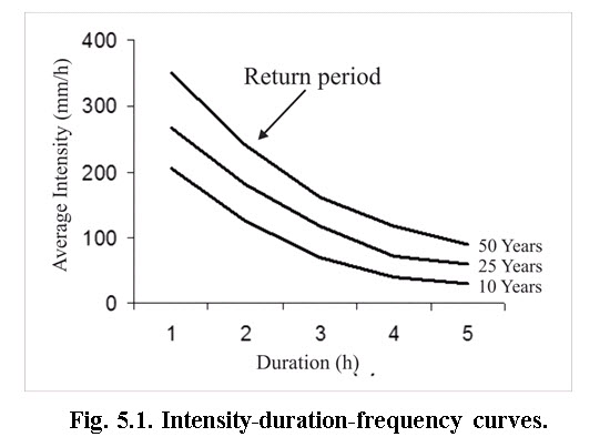
 Fig. 5.1 shows a typical variation of intensity with duration and return period. Typical values of the constants, K, T, a and n for few Indian location are given in Table 5.4.

 Table 5.4. Values of constant for IDF relationship

Station	K	x	a	n
Bhopal	6.93	0.189	0.50	0.878
Nagpur	11.45	0.156	1.25	1.032
Chandigarh	5.82	0.160	0.40	0.75
Bellary	6.16	0.694	0.50	0.972
Raipur	4.68	0.139	0.15	0.928

(Based on the studies of CSWCRTI, Dehradun)

 Example 5.1: Consider a watershed of certain area. Let’s assume there is a rain gauge station and the watershed is meteorologically homogeneous. The rainfall data for last 30 years are analyzed and presented in Table 5.5.

 Table 5.5: Rainfall data corresponding to different RI and duration at a sample station

Return Period (years)	Excess rainfall (mm/hr)
	5-min	10-min	15-min	30-min	60-min	90-min
2	12.8	16.3	20.9	28.4	36.1	42.3
5	17.6	24.2	29.8	38.4	47.3	58.2
10	24.3	30.1	38.5	44.9	58.0	67.8
20	39.1	35.1	43.8	51.2	59.4	71.4
25	45.2	50.3	54.2	57.3	61.3	75.6
50	55.9	59.3	66.3	71.2	76.3	81.7
100	71.6	78.5	87.3	91.4	96.7	102.5

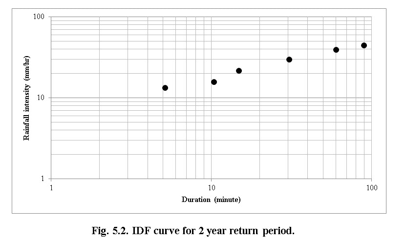
 The IDF curves are established using double-log paper with abscissa as intensity and ordinates as duration (minutes). The points are plotted on the log-log paper for return period such that one IDF respective to return period.

Plot the IDF curve for rainfall data given above

 Solution:

Take a log-log paper. Plot the points for 12.8, 16.3, 20.9, 28.4, 36.1 and 42.3 mm/hr intensity respective to 5, 10, 15, 30, 60 and 90 minute duration corresponding to 2 year return period on this log paper as shown in Fig. 2. Follow the same procedure for the other return periods.

5.5 Limitations of Rational Method

When used correctly, the Rational method can be a very effective tool at estimating runoff.  However, several limitations should be considered before using this method.

• The Rational method assumes that the drainage basin characteristics are fairly homogeneous. If the watershed being considered includes a variety of surfaces, such as paved areas, wooded areas, and agricultural fields, then another method should be selected.

• The Rational method is less accurate for larger areas and is not recommended for drainage areas larger than 80 ha.

• The only output from Rational method is a peak discharge (the method provides only an estimate of a single point on the runoff hydrograph).

• The average rainfall intensities used in the formula have no time sequence relation to the actual rainfall pattern during the storm.

 5.5.1 Assumptions

• For this method, it is assumed that a rainfall duration equal to the time of concentration results in the greatest peak discharge.

• The time of concentration is the time required for runoff to travel from the most distant point of the watershed to the outlet.  Intuitively, once a rainfall event begins the amount of water flowing out of the watershed will begin to increase until the entire watershed is contributing water, at the time of concentration. 

• Rainfall intensity is uniform over duration of time equal to or greater than the time of concentration. Under steady rainfall intensity, the maximum discharge will occur at the watershed outlet at the time when the entire area above the outlet is contributing runoff

• Rational coefficients are independent of the intensity of the rainfall.

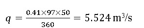
 Example 5.2: Determine the design peak runoff rate for a 50-year return period storm from a 50-ha watershed, with the following characteristics:

Area(ha)	Topography, per cent slope	Soil group	Land use, treatment, and hydrologic condition
30	5-10	C	Row crop, contoured, good
20	10-30	B	Woodland, good

 The maximum length of flow is 600 m and the difference in elevation along the path is 3 m.

 Solution:

The watershed gradient can be calculated as (3/600) ×100 = 0.5 %

 The time of concentration (T_c) is calculated by using the Eq. 5.3 as follows:                     

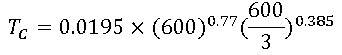
                               T_c = 20 min.

 For a 50-year return period of the study area, the rainfall intensity for duration equal to the time of concentration of the watershed can be calculated from the Eq. 5.4 is 97 mm/h 

 The runoff coefficients C from Table 5.1 for row crop, good practice, and woodland are 0.56 and 0.10, respectively, and the factor correcting hydrologic soil group B to group C for the 30-ha subarea from Table 5.2 is 1.09

 The runoff coefficient is calculated as follows

  ....  (from Eq. 5.2)

 Thus, the design peak runoff rate is calculated by using Eq. 5.1 as

 

 Example 5.3: The land use pattern of a watershed is given in the following table. The hydrologic soil group of the watershed is B. Calculate the peak rate of runoff for rainfall intensity of 100 mm/h for the duration of Tc of watershed.

Land Use classification	Crop and management practice	Area(ha)
Land use A	Forest with matured woodland	25
Land use B	Row crop, good practice	30
Land use C	Small grain, good practice	20
Land use D	Grassland with rotating species, good practice	10

 Solution:

From the Table 5.1, the composite runoff coefficient for the given watershed is calculated as

 

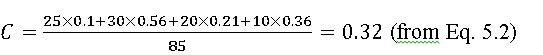
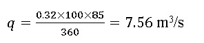
So, the peak runoff rate is calculated by using the Eq. 5.1 as

 

 Example 3: A catchment has an area of 500 ha. The average slope of the land surface is 0.5% and the maximum travel depth of rainfall in the catchment is approximately 2 km. The maximum depth of rainfall in the area with a return period of 25 years is as tabulated below:

Time duration (min)	5	10	15	20	25	30	40	60
Rainfall depth (mm)	15	25	32	45	50	53	60	65

 Consider that 200 ha of the catchment area has cultivated sandy loam soil (C = 0.2) and 300 ha has light clay cultivated soil (C = 0.7). Determine the peak flow rate of runoff by using the Rational method.

 Solution:

The time of concentration (T_c) is calculated by using the Eq. 5.3 as follows:

                      

                        T_c = 52.21 min.

 The maximum rainfall depth for 52.21 min duration would fall between the period 40-60 min and is located at 12.21 min after the 40 min period at which the maximum rainfall depth is 60 mm, as from the Table provided/ available data.

 The rainfall depth during the 12.21 min period 

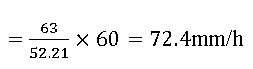
 Therefore, at 52.21 min duration, the rainfall depth = 60 + 3 = 63 mm.

 The average rainfall intensity = maximum rainfall depth/T_c (during the period of T_c)

                                 

 The runoff coefficient is calculated as follows

 

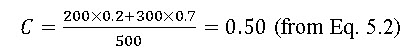
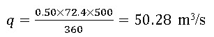
 The Rational method of predicting peak runoff rate is calculated by using Eq. 5.1 as

References

• Das. G. (2000). Hydrology and Soil Conservation Engineering, Prentice Hall of

• India Private Ltd., New Delhi, 2000

• Michael A.M., and Ojha, T. P. (2006). Principles of Agricultural Engineering,

• Volume II, 3^rd ed., Jain Brothers, New Delhi

• Schwab, G.O., Fangmeier, D.D., Elliot, W.T., and Frevert, R.K. (1993). Soil and

• Water Conservation Engineering,4^thed., John Wiley & Sons,New York.

• Subramanya, K. (1994). Engineering Hydrology, Tata McGraw –Hill Publishers,

• New Delhi, 1994.

• Suresh R. (2007). Soil and water conservation engineering, 2^nd ed., Standard

• Publishers Distributors, Delhi.

 

Internet References

• http://www.ctre.iastate.edu/pubs/stormwater/documents/2C-4RationalMethod.pdf

• http://docs.bentley.com/en/HMStormCAD/Bentley_WaterGEMS_Help-10-014.html

• http://www.dcr.virginia.gov/stormwater_management/documents/Chapter_4.pdf

• http://www.nilebasin- journal.com/Volumes/Volume4/issue6/generation%20of%20rainfall.pdf

Suggested reading

• Das. G. (2000). Hydrology and Soil Conservation Engineering, Prentice Hall of

• India Private Ltd., New Delhi, 2000

• Michael A.M., and Ojha, T. P. (2006). Principles of Agricultural Engineering,

• Volume II, 3^rd ed., Jain Brothers, New Delhi

• Subramanya, K. (1994). Engineering Hydrology, Tata McGraw –Hill Publishers,

• New Delhi, 1994

• Suresh R. (2007). Soil and water conservation engineering, 2^nd ed., Standard

• Publishers Distributors, Delhi.