Soil & Water Conservation Structures 3(2+1)

Lesson 6. Runoff Estimation

6.1 SCS-CN Method

The SCS curve-number (SCS-CN) method was developed by the Soil Conservation Service for estimating runoff volume (SCS, 1969). It is widely used to estimate runoff from small-to medium-sized watersheds. It relies on only one parameter, i.e., curve number CN.

 6.1.1 Basic Concepts

Runoff volume V_q is the total volume of runoff water occurring over a period of time expressed as

                                    

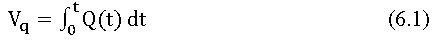
 Where Q_t is the discharge at time t.

 This runoff volume resulted due to the precipitation occurred on a drainage basin. The Curve Number Method is based on two phenomena. The fundamental hypotheses of this method are:

1. Runoff starts after an initial abstraction I_a(mainly consists of interception, surface/depression storage, and infiltration) has been satisfied,
2. The ratio of actual retention of rainfall to the potential maximum retention S is equal to the ratio of direct runoff to rainfall minus initial abstraction.

 To describe the phenomena, mathematically the relationship can be expressed as:

                                     

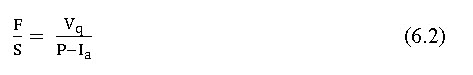
 Where F is the actual retention, S is the potential maximum retention, P is the accumulated rainfall depth, I_a is the initial abstraction.

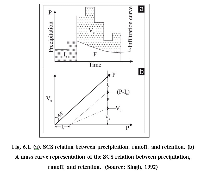
 Fig. 1(a) and (b) shows the above relationship for certain values of the initial abstraction and potential maximum retention. After runoff has started, the actual retention equals to rainfall minus initial abstraction and runoff.

 Thus,                                      

      F = P - I_a – V_q                                      (6.3)

 Putting Eq. (6.3) in (6.2) gives

                                       

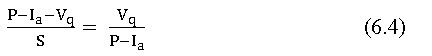
 Thus,

                                                                                      

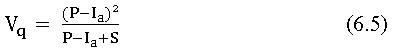
To eliminate the need to estimate the two variables I_a and S in Eq. (6.5), a regression analysis was made on the basis of recorded rainfall and runoff data from small drainage basins (SCS 1972). The following average relationship was found

                                                                                              

 Physically it means that for a given storm, 20% is the initial abstraction before the start of runoff. For Indian conditions,

                                                

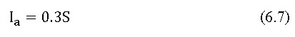
 The value of I_a is subjected to corrections based on different AMC conditions and soil type and can vary from 0.1S to 0.4S. For red soil (Alfisol) and black soil (Vertisol), I_a value is taken as 0.15S and 0.3S respectively (Dhruvanarayana, 1993).

 Combining Eqns. (5) and (6) gives

           

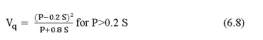
 The Eq. (6.8) is the rainfall-runoff relationship used in the CN Method. It allows the runoff depth to be estimated from rainfall depth, given the value of the potential maximum retention S.

 6.1.2 Estimation of S

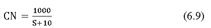
Estimation of the potential maximum retention, S in a watershed is very difficult as it depends on the characteristics of soil-vegetation-land use (SVL) complex and antecedent soil-moisture conditions. The Soil Conservation Service (SCS) expressed S as a function of curve number as:

 

                                 

 

or                                                                                    

 

Where CN is a dimensionless number ranging from 0-100 as shown in Fig. (2), S is in inches. For SI unitof S (mm) the Eq. (6.9) is modified to

 

                                                                                       

 

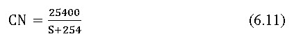
The usual practice to compute runoff, V_q, first compute S for given CN values (using Eq.6.10) and then substitute S in the (Eq. 6.8).

 For example: For paved areas, when CN equals 100, S becomes zero (Eq.6.10) and all rainfall will become runoff (Eq.6.8). In contrasts, for highly permeable, flat lying soils, when CN equals zero, S will go to infinity, (Eq. 6.10), hence, all rainfall will infiltrate and there will be no runoff. In drainage basins, the reality will be in between these two conditions.

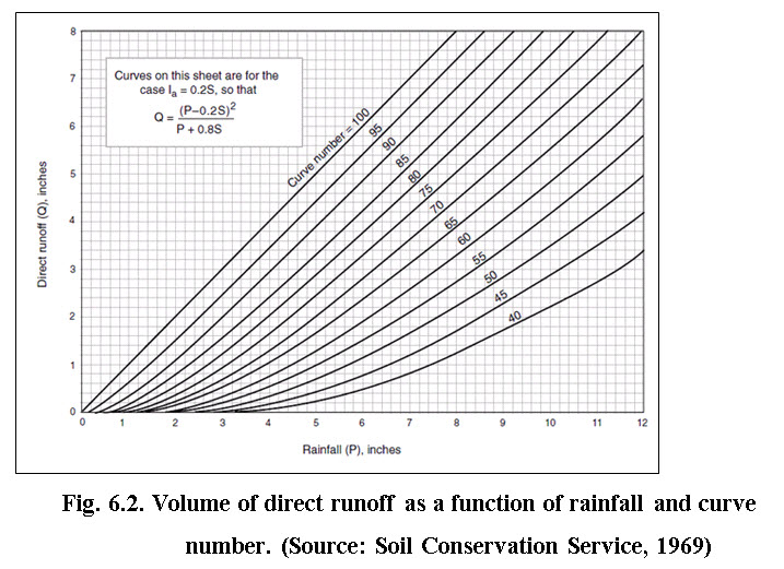
To estimate the volume of direct runoff Eq. (6.8) and (6.10) can be used for the known amount of precipitation and curve number. The SCS (1969) developed a graphical solution as shown in Fig. 6.2 of these equations. Either of these approaches can be made to estimate the volume of surface runoff.

6.1.3 Limitations of SCS CN Method

The followings are the limitations of SCS curve number method:

(i) The soil group of the basin should have uniform hydrologic characteristics.

(ii) Rainfall should be uniform and distributed uniformly over the basin area.

(iii) All other hydrologic characteristics should be uniform.

 As most of the drainage basins do not satisfy the above assumptions, this curve number method over-predicts by a large magnitude.

6.1.4 Peak Flow Rate Determination using SCS-CN

The SCS-CN estimates the peak runoff rate by using the following equation developed by Ogrosky and Mockus (1957) by using the 6-hour rainfall as the design frequency of small watersheds.

 

                         

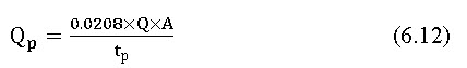
 Where Q_p is peak rate of runoff in m³/s, Q is the runoff depth in cm, A is area of watershed in ha, t_p is the time to peak in hour. Time to peak, t_p, is estimated from time of concentration, t_c, in hour, using the following equation:

 

                   

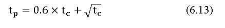
 The time of concentration, t_c can be determined by the CN Method using the following equation (Schwab et al., 1993):

 

                                                                                   

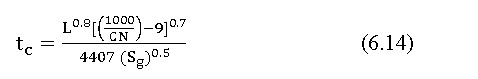
 Where L is the longest flow length in metre, CN is the curve number, S_g is the average slope of the watershed in percent.

 6.2 Hydrologic Soil Group

The CN values are highly dependent on the soil surface. The soil surfaces are grouped into 4 classes which are known as hydrologic soil groups. These are classified into 4 classes on the basis of runoff potential of the surface and are described below:

1.   Group-A: (Lowest Runoff Potential): Soils in this group have the lowest runoff potential(high infiltration rates) even when thoroughly wetted and consist chiefly of deep, well to excessively drained sands or gravels. These soils have a high rate of water transmission.
2.   Group-B: (Moderately Low Runoff Potential): Soils having moderate infiltration rates when thoroughly wetted and consisting chiefly of moderately deep to deep, well drained to moderately well-drained soils with moderately fine to moderately coarse textures. These soils have a moderate rate of water transmission.
3.   Group-C: (Moderately high Runoff Potential): Soils having slow infiltration rates when thoroughly wetted and consisting chiefly of soils with a layer that impedes downward movement of water, or soils with moderately fine to fine texture.  These soils have a slow rate of water transmission.
4.   Group-D: (Highest Runoff Potential): Soils having very slow infiltration rates when thoroughly wetted and consisting chiefly of clay soils with a high swelling potential, soils with a permanent high water table, soils with a clay pan or clay layer at or near the surface and shallow soils over nearly impervious material.  These soils have a very slow rate of water transmission.

 The characteristics and ranges of infiltration rates of the soil groups are described in Table 6.1.

 Table 6.1. Soil group classification (Source: Singh, 1992)

Group	Soil characteristics	Minimum infiltration rate(in./h)
A	Deep sand, deep loss, and aggregated silts	0.3-0.45
B	Shallow losses and sandy loam	0.15-0.30
C	Clay loams, shallow sandy loam, soils in organic content, and soils usually high in clay	0.05-0.15
D	Soils that swell upon wetting, heavy plastic clays, and certain saline soils	0-0.05

 

6.3 Antecedent Moisture Condition (AMC)/Antecedent Runoff Conditions

Antecedent Moisture Condition is the preceding relative moisture of the pervious surfaces prior to the rainfall event. AMC is an important factor in runoff process because it reflects the relative saturation of the soil, which influences the infiltration process. AMC is also known as Antecedent Runoff Condition (ARC). Antecedent moisture considered as low, when there has been little preceding rainfall and high, when there has been considerable preceding rainfall prior to the rainfall event under consideration. For purpose of practical application, SCS suggests three levels of AMC as follows:

AMC-I: Soils are dry but not to wilting point. Satisfactory cultivation has taken place.         

AMC-II: Average conditions.

AMC-III: Sufficient rainfall has occurred within the immediate past 5 days. Saturated soil conditions prevail.

 The limits of these three AMC classes, based on total rainfall magnitude in the previous 5 days, are given in Table 6.2. It is to be noted that the limits also depend upon the seasons like growing season and dormant season are considered.

 Table 6.2. AMC for determining the value of CN

 

AMC Type	Total Rain in Previous 5 days
	Dormant season	Growing Season
I II III	Less than 13 mm 13 to 28 mm More than 28 mm	Less than 36 mm 36 to 53 mm More than 53 mm

(Source: http://www.mhhe.com/subramanya/eh3e)

6.3.1 Runoff Curve Number Determination

The determination of the CN value for a watershed is a function of soil characteristics, hydrologic condition and cover or land use. CN values for Hydrological soil cover (Under AMC-II conditions) for Indian conditions are given in Table 6.3. For watersheds with multiple soil types or land uses, an area-weighted CN should be calculated. Table 6.4 shows the CN values for fully developed and developing urban areas. For AMC condition I and III, the multiplying factors given in Table 6.5 are used to convert the curve number for respective AMC conditions at interval of 10. For other values of CN, multiplication factorcan be obtained after interpolation.

 Table 6.3. Runoff curve numbers (AMC-II) for the Indian conditions

Sl. No	Landuse	Treatment/Practice	Hydrologic condition	Hydrologic soil group
				A	B		C	D
1	Cultivated	Straight row	-------	76	86	90		93
		Contour	Poor	70	79	84		88
			Good	65	75	82		86
		Contour and terraced	Poor	66	74	80		82
			Good	67	75	81		83
		Bunded	Poor	59	69	76		79
			Good	95	95	5		95
		Paddy(rice)	-----
2	Orchards	With under stony     cover	-----	39	53	67		71
		Without under Stony cover	-----	41	55	69		73
3	Forest	Dense	-----	26	40	58		61
		open	-----	28	44	60		64
		shrubs		33	47	64		67
4	Pasture	------	Poor	68	79	86		89
			Fair	49	69	79		84
			Good	39	61	74		80
5	Wasted Land	------	-----	71	80	85		88
6	Hard surface	------	------	77	86	91		93

(Source: http://www.ijest.info/docs)

 Table 6.4. Runoff curve number (values for fully developed and developing urban areas)

Cover description		Curve numbers for hydrologic soil group
Cover type and hydrologic condition	Average % impervious area	A	B	C	D
Open space (lawns, parks, golf courses, cemeteries, etc.): Good condition (grass cover > 75%) Fair condition (grass cover 50% to 75%) Poor condition (grass cover less than 50%)		39 49 68	61 69 79	74 79 86	80 84 89
Impervious areas: Paved parking lots, roofs, driveways, compacted gravel, etc. (excluding right-of-way)		98	98	98	98
Small open spaces within developments or ROW:		72	82	87	89
Streets and roads: Paved: curbs and storm sewers (including right-of-way) Paved: open ditches (including right-of-way)  Gravel (including right-of-way) Dirt (including right-of-way)		90 83 76 72	93 89 85 82	95 92 89 87	97 93 91 89
Urban districts: Commercial and business Industrial	85 72	89 81	92 88	94 91	95 93
Residential districts by average lot size:      1/8 acre or less (townhouses) 1/4 acre  1/3 acre 1/2 acre 1 acre 2 acres	65 38 30 25 20 12	77 61 57 54 51 46	85 75 72 70 68 65	90 83 81 80 79 77	92 87 86 85 84 82
Developing urban areas: Newly graded areas (pervious areas only, no vegetation)		77	86	91	94

(Source: www.springfieldmo.gov by Chow et al. 1988)

 

Table 6.5. Multiplication factor for converting AMC II to I and III conditions

Curve number/ weighted curve number for AMC II	Factors to convert from AMC II to
	AMC I	AMC II
10	0.40	2.22
20	0.45	1.85
30	0.50	1.67
40	0.55	1.50
50	0.62	1.40
60	0.67	1.30
70	0.73	1.21
80	0.79	1.14
90	0.87	1.07
100	1.00	100

(Source: Technical Bulletin 3/2012, CRIDA, Hyderabad)

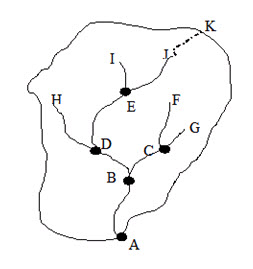
 Example 6.1: In a watershed shown in the figure below, a water harvesting structure is planned to construct at point A. The catchment area to this point is 137 ha, out of which 78 ha area is under groundnut cultivated in straight row, 29 ha area is under fodder cultivation and remaining area is covered with tree plantation. The prevailing soil type of the catchment is vertisol and rainfall analysis suggested 86.4 mm 6-hours duration rainfall can be expected for 25 years return period and experience frequent rainfall in the season. Determine the potential runoff volume that can be generated from this catchment.

 

 

Solution:

Since the soil type is vertisol (black soil), the hydrologic soil group of this catchment is D. Using Table 3 the CN values for ground nut cultivation, fodder cultivation and plantation would be 93, 80 and 73 respectively.

Hence the weighted curve number would be

 

    = (93×78+80×29+73×30)/137 = 85.86 or 86(say)

 

Since the area experience frequent rainfall, the AMC conditions would be III.

By linear interpolation, the multiplying factor for CN value of 86 would be 1.1. Hence the converted CN value would be 86×1.1 = 95.6

 

Now, compute S, we know that   

 Therefore,             S = 11.7                

 

Since the soil type is black soil, I_a will be equal to 0.25S                        

 

Now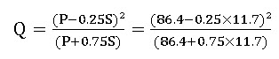                              

                                      = 73.2 mm

Total volume of storage structure when all the runoff to be stored will be 10ha-m approximately.

References

• Chow, V. T., D. R. Maidment, and L.W. Mays. (1988). Applied Hydrology. McGraw-Hill, Inc.

• Das, Ghanshyam. (2000). Hydrology and Soil Conservation Engineering, Prentice Hall of India Private Ltd., New Delhi, India.

• Dhruva Narayana, V. V. (1993). Soil and Water Conservation Research in India, ICARKrishiAnusandhanBhavan, Pusa, New Delhi, India.

• Michael, A.M. and Ojha, T.P. (2006). Principles of Agricultural Engineering, Vol. II, Jain Brothers, New Delhi, India.

• Schwab, G.O., D.D. Fangmeier, W.T. Elliot, R.K. Frevert. (1993). Soil and Water Conservation Engineering, John Wiley & Sons, New York, United States.

• Garg, S.K. (2004). Irrigation Engineering and Hydraulic Structures, Khanna Publications, New Delhi, India.

• Subramanya, K. (1994). Engineering Hydrology, Tata McGraw –Hill Publishers, New Delhi, India.

• Suresh, R. (2007). Soil and Water Conservation Engineering, Second edition, Standard Publisher Distributors, Delhi, India.

• Technical bulletin 3/2012 Farm ponds: A climate resilient technology for Rainfed agriculture – Planning design and construction. Central Research Institute for Dryland Agriculture, Hyderabad, AP, India.

• USDA Natural Resources Conservation Service, 210-VI-NEH, (2004). Part 630 Hydrology National Engineering Handbook.

• Soil Conservation Service, USDA. Hydrology, Section 4. (1964). National Engineering Handbook, Washington, D.C., Revised Edition.

Internet references:

• http://colleges.ksu.edu.sa/Papers/Papers/scs-cn1.pdf as accessed on 3/10/2013

• http://www.czen.org/files/czen/ElhakeemM_09WRM.pdf as accessed on 3/10/2013

• http://pubs.usgs.gov/wsp/wsp2363/pdf/wsp_2363_a.pdf as accessed on 3/10/2013

• http://www.hydrol-earth-syst-sci.net/16/1001/2012/hess-16-1001-2012.pdf as accessed on 3/10/2013

• http://www.crida.in/Pubs/Farm%20ponds%20technical%20bulletin%20201.pdf  as accessed on 3/10/2013

• http://edepot.wur.nl/183157 as accessed on 3/10/2013

Suggested Readings

• Chow, V. T., D. R. Maidment, and L.W. Mays. (1988). Applied Hydrology.McGraw-Hill, Inc.

• Das Ghanshyam. (2000). Hydrology and Soil Conservation Engineering, Prentice Hall of India Private Ltd., New Delhi, India.

• Garg, S.K. (2004). Irrigation Engineering and Hydraulic Structures, Khanna Publications, New Delhi, India.

• Subramanya, K. (1994). Engineering Hydrology, Tata McGraw –Hill Publishers, New Delhi, India.

• Suresh, R. (2007). Soil and Water Conservation Engineering, Second edition, Standard Publisher Distributors, Delhi, India.