Reservior & Farm Pond Design 3(2+1)

Lesson 14 Flow Net

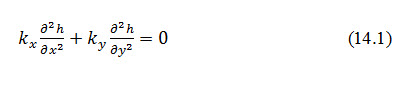
Where, h(x, y) = distribution of the total energy head within and on the boundaries of a flow region, and&= coefficients of permeability in x and y directions, respectively. If the flow system is isotropic,= , and Eqn. (14.1) reduces to

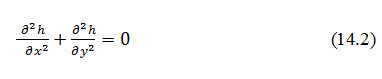
Equation (14.2), called Laplace’s equation, is the governing relationship for steady state, laminar-flow conditions (Darcy’s law is valid). The general body of knowledge relating to Laplace’s equation is called potential theory. Correspondingly, incompressible steady state fluid flow is often called potential flow.

The introduction of the velocity potential fis defined as

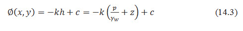
Where, h = total head, = pressure head, z = elevation head, and C = arbitrary constant. It should be apparent that, for isotropic conditions,

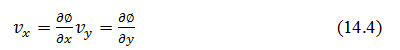
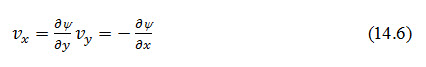
Where &= components of the velocity in the x and y directions, respectively.

and Eqn. (14.2) will produce,

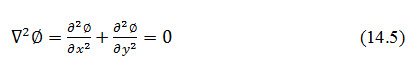
The particular solutions of Eqns. (14.2) or (14.5) that yield the locus of points within a porous medium of equal potential, curves along which h(x, y) or f (x, y) are equal to constants, are called equipotential lines.

In analyses of flow through porous media, the family of flow paths is given by the function (x, y), called the stream function, defined in two dimensions as:

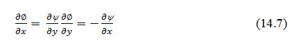
Equating the respective potential and stream functions of and produces

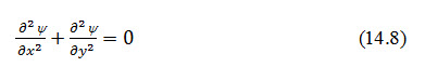
Differentiating the first of these equations with respect to y and the second with respect to x and adding, we obtain Laplace’s equation:

Examining the significance of this relationship, a little more discussion of the physical meaning of the stream function is presented in following paragraphs. Consider AB of Fig. 14.1as the path of a particle of water passing through point P with a tangential velocity v.

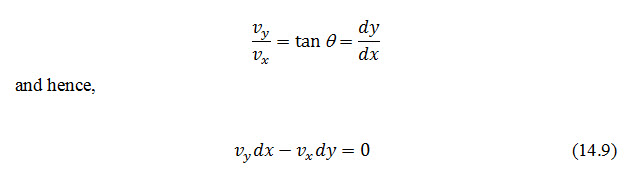
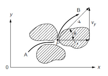
Fig.14.1. Path of flow.

(Source: Harr, 2003)

Substituting Eqn. (14.6), it follows that

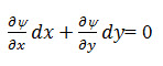
Which states that the total differential dy= 0 andy(x,y) = constant

Thus we see that the family of curves generated by the function y(x,y) equal to a series of constants are tangent to the resultant velocity at all points in the flow region and hence define the path of flow. The potential [f= – kh+ C] is a measure of the energy available at a point in the flow region to move the particle of water from that point to the tail water surface. Recall that the locus of points of equal energy, say, f (x, y) = constants, are called equipotential lines.

The total differential along any curvef(x, y) = constant produces

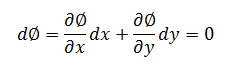
Substituting for ∂Ø∂x and ∂Ø∂y from Eqs. (14.4), we have,

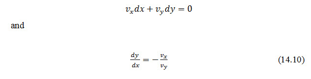
Noting the negative reciprocal relationship between their slopes, Eqns. (14. 9) and (14.10) indicate the families of streamlines,y(x, y) = constants and equipotential lines f (x, y) =constants, intersect each other at right angles within the flow domain. It is customary to signify the sequence of constants by employing a subscript notation, such as f (x, y) = f_i, y(x, y) = y_j (Fig. 14.2). As only one streamline may exist at a given point within the flow medium, streamlines cannot intersect with one another. Consequently, if the medium is saturated, any pair of streamlines acts to form a flow channel between them. Consider the flow between the two streamlines yand y+ dy in Fig. 14.3; represents the resultant velocity of flow. The quantity of flow through the flow channel per unit length normal to the plane of flow is.

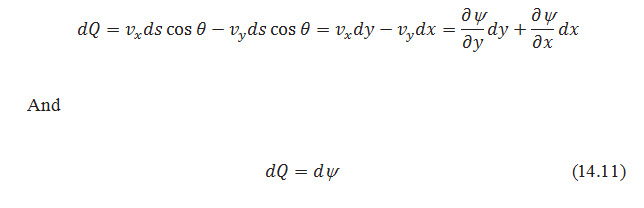
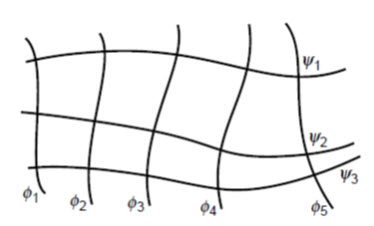
Fig. 14.2. Streamlines and equipotential lines.

(Source: Harr, 2003)

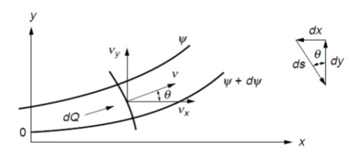
Fig. 14.3. Flow between  streamlines.

(Source: Harr, 2003)

Hence the quantity of flow (also called the discharge quantity) between any pair of streamlines is a constant whose value is numerically equal to the difference in their respective y values. Thus, once a sequence of streamlines of flow has been obtained, with neighboring y values differing by a constant amount, their plot will not only show the expected direction of flow but the relative magnitudes of the velocity along the flow channels; that is, the velocity at any point in the flow channel varies inversely with the streamline spacing in the vicinity of that point.An equipotential line was defined previously as the locus of points where there is an expected level of available energy sufficient to move a particle of water from a point on that line to the tail water surface.

Thus, it is convenient to reduce all energy levels relative to a tail water datum. For example, a piezometer located anywhere along an equipotential line, say at 0.75h in Fig. 14.4, would display a column of water extending to a height of 0.75h above the tail water surface. Of course, the pressure in the water along the equipotential line would vary with its elevation.

14.2 Flow Nets

The graphical representation of special members of the families of streamlines and corresponding equipotential lines within a flow region form a flow net. The orthogonal network represents such a system (Fig. 14.5). Although the construction of a flow net often requires tedious trial-and-error adjustments, it is one of the more valuable methods employed to obtain solutions for two-dimensional flow problems. Of additional importance, even a hastily drawn flow net will often provide a check on the reasonableness of solutions obtained by other means.

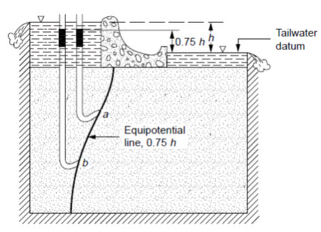
Fig. 14.4. Pressure head along equipotential line.

(Source: Harr, 2003)

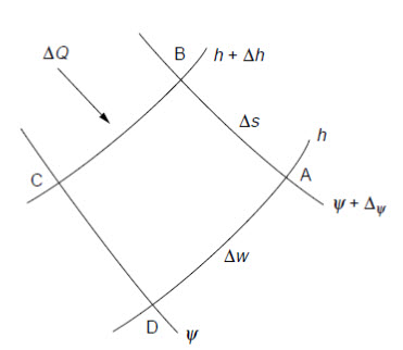
Fig. 14.5. Flow net at a point.

(Source: Harr, 2003)

14.3 Characteristics of Flow Nets

1. Flow lines or stream lines represent flow paths of particles of water.

2. Flow lines and equipotential line are orthogonal to each other.

3. The area between two flow lines is called a flow channel.

4. The rate of flow in a flow channel is constant.

5. Flow cannot occur across flow lines.

6. An equipotential line is a line joining points with the same head.

7. The velocity of flow is normal to the equipotential line.

8. The difference in head between two equipotential lines is called the potential drop or head loss (dh).

9. A flow line cannot intersect another flow line.

10. An equipotential line cannot intersect another equipotential line.

Key words: Streamline, Equipotential line, Discharge, Flow net

References

• Harr, M. E. (2003). Ground Water and Seepage (Edited by Chen, W. F.).The Civil Engineering Handbook. Second  Edition. CRC press LLC.

• Suresh, R. (2002). Soil and Water Conservation Engineering. Fourth Edition. Standard Publishers. 

• http://elearning.vtu.ac.in/10/enotes/06CV64/Unit4-KVV.pdf

Suggested Readings

• Garg, S. K. (2011). Irrigation Engineering and Hydraulic Structures. Twenty fourth Revised Edition, Khanna Publication.

• http://faculty.washington.edu/jdlund/classes/CEE345/FlowNets/constructing_flow_nets_humboldt_directionsonly.pdf

• http://en.wikipedia.org/wiki/Flownet

• http://faculty.uml.edu/ehajduk/Teaching/14.333/documents/14.3332013FlowNets.pdf

• http://eng.upm.edu.my/webkaw/coursenotes/kaw4313/FlowNets.htm