Site pages
Current course
Participants
General
MODULE 1. Analysis of Statically Determinate Beams
MODULE 2. Analysis of Statically Indeterminate Beams
MODULE 3. Columns and Struts
MODULE 4. Riveted and Welded Connections
MODULE 5. Stability Analysis of Gravity Dams
Keywords
LESSON 9. Force Method: Three-Moment Equation
Beams that have more than one span are called continuous beam. In this lesson a general equation based on method consistent deformation (lesson 8) is derived and applied to solve continuous beam. This equation gives a relationship among the bending moments at three consecutive supports and hense often called as Three-Moment Equation.
9.1 Derivation of Three-Moment Equation
Consider a arbitrarily loaded continuous beam in which A, B and C are three consicutive support as shwon in Fgiure 9.1.
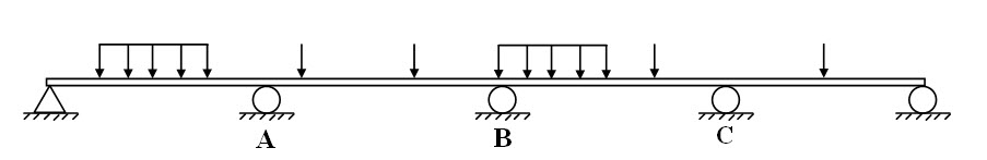
Fig. 9.1.
Let LAB, IAB and EAB, LBC, IBC nd EBC are span length, second moment of area and Young’s modulus coresponding to span AB and BC respectively. This is an indeterminate beam which may be made statically determinate by releasing moment constraint (inserting hinge) at A, B and C. Therefore MA, MB and MC are the redundatn moments. The basic determinate structure is shwon in Figure 9.2.
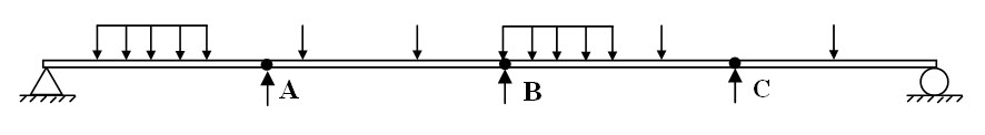
Fig. 9.2.
Deflected shape of the span AB and BC due to external loading and the redundant moments are shwon in Fgure 9.3a-b.
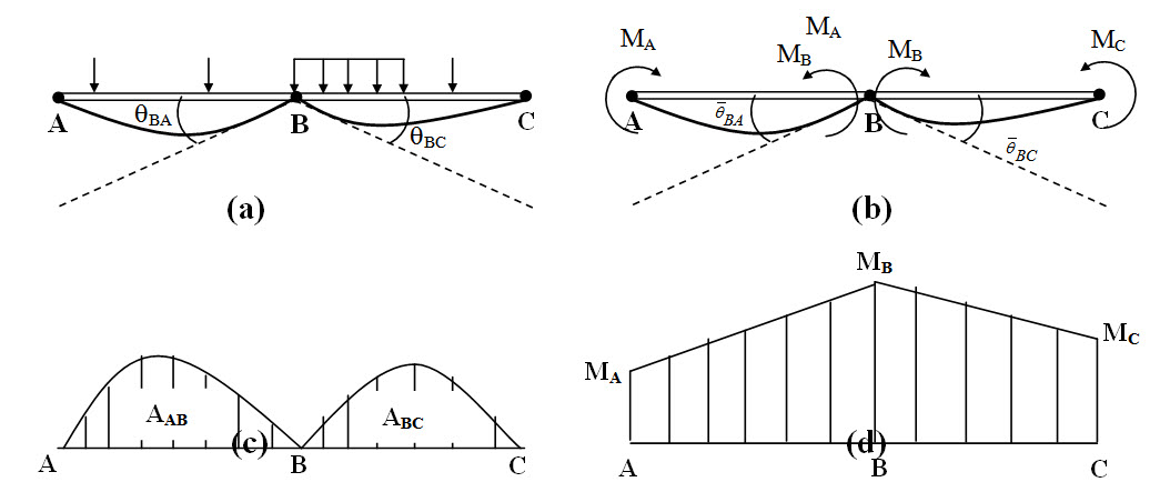 Fig. 9.3.
Slopes at θBA, θBC due to external loading (Figure 9.3a) and \[{\bar \theta _{BA}}\] , \[{\bar \theta _{BC}}\] due to redundant momoment (Figure 9.3a) may be obtaind moment-area method discussed in lesson 5. Bending moment diagrams for each span are shwon in Figure 9.3c-d.
\[{\theta _{BA}} = {{{{{{{{\rm{Moment of }}M} /{EI{\rm{ diagram between A and B about A}}}}} \over {{{\rm{L}}_{{\rm{AB}}}}}} = {{{A_{AB}}{x_{AB}}} \over {{E_{AB}}{I_{AB}}{L_{AB}}}}\]
\[{\theta _{BC}} = {{{{{{{{\rm{Moment of }}M} /{EI{\rm{ diagram between B and C about C}}}}} \over {{{\rm{L}}_{{\rm{AB}}}}}} = {{{A_{BC}}{x_{CB}}} \over {{E_{BC}}{I_{BC}}{L_{BC}}}}\]
Similarly, \[{\bar \theta _{BA}}\] and \[{\bar \theta _{BC}}\] may be obtained as,
\[{\bar \theta _{BA}} = {1 \over {{L_{AB}}}}\left[ {{{{M_A}{L_{AB}}} \over {E{I_{AB}}}}{{{L_{AB}}} \over 2} + {1 \over 2}{{\left( {{M_B} - {M_A}} \right){L_{AB}}} \over {E{I_{AB}}}}{{2{L_{AB}}} \over 3}} \right] = {{{M_A}{L_{AB}}} \over {6{E_{AB}}{I_{AB}}}} + {{{M_B}{L_{AB}}} \over {3{E_{AB}}{I_{AB}}}}\]
\[{\bar \theta _{BC}} = {1 \over {{L_{BC}}}}\left[ {{{{M_C}{L_{BC}}} \over {E{I_{BC}}}}{{{L_{BC}}} \over 2} + {1 \over 2}{{\left( {{M_B} - {M_C}} \right){L_{BC}}} \over {E{I_{BC}}}}{{2{L_{AB}}} \over 3}} \right] = {{{M_C}{L_{BC}}} \over {6{E_{BC}}{I_{BC}}}} + {{{M_B}{L_{BC}}} \over {3{E_{BC}}{I_{BC}}}}\]
Now, compatibility condition at B says, the relative rotation at B is zero.
Therefore,
\[{\theta _{BA}} + {\theta _{BC}} + {\bar \theta _{BA}} + {\bar \theta _{BC}}=0\]
\[\Rightarrow {{{A_{AB}}{x_{AB}}} \over {{E_{AB}}{I_{AB}}{L_{AB}}}} + {{{A_{BC}}{x_{CB}}} \over {{E_{BC}}{I_{BC}}{L_{BC}}}} + {{{M_A}{L_{AB}}} \over {6{E_{AB}}{I_{AB}}}} + {{{M_B}{L_{AB}}} \over {3{E_{AB}}{I_{AB}}}} + {{{M_C}{L_{BC}}} \over {6{E_{BC}}{I_{BC}}}} + {{{M_B}{L_{BC}}} \over {3{E_{BC}}{I_{BC}}}}=0\]
\[\Rightarrow {{{M_A}{L_{AB}}} \over {{E_{AB}}{I_{AB}}}} + 2{M_B}\left( {{{{L_{AB}}} \over {{E_{AB}}{I_{AB}}}} + {{{L_{BC}}} \over {{E_{BC}}{I_{BC}}}}} \right) + {{{M_C}{L_{BC}}} \over {{E_{BC}}{I_{BC}}}}=-{{6{A_{AB}}{x_{AB}}} \over {{E_{AB}}{I_{AB}}{L_{AB}}}} - {{6{A_{BC}}{x_{CB}}} \over {{E_{BC}}{I_{BC}}{L_{BC}}}}\]
The above equation is known as the Three-Moment Equation.
9.1.2 Three-Moment Equation with Support Settlement
In the above form of Three-Moment Equation it was assumed that the support reactions and internal forces in the beam are induced only due to external load. However, sometime movement of joints, for example support settlement may take place and if it happens, its effect has to be considered in the analysis. In this section, a generalised Three-Moment Equation including the effect of support settlement is derived.
Consider the continuous beam given in Figure 9.1. Additionally suppose support A, B and C have settled to position A¢, B¢ and C¢ by amounts dA, dB and dC respectively as shwon in Figure 9.4.
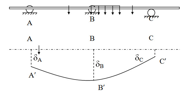
Fig. 9.4.
Deflection of B with respect to A, dBA = dB – dA
Deflection of B with respect to C, dBC = dB – dC
Relative deflection at B with respect to A and C cause rotation at B which may be obtained as,
\[{\hat \theta _{BA}}=-{{{\delta _{BA}}} \over {{L_{AB}}}}\] and \[{\hat \theta _{BC}}=-{{{\delta _{BC}}} \over {{L_{BC}}}}\]
Now apply the compatibilty condition at B,
\[{\theta _{BA}} + {\theta _{BC}} + {\bar \theta _{BA}} + {\bar \theta _{BC}} + {\hat \theta _{BA}} + {\hat \theta _{BC}}=0\]
\[\Rightarrow {{{M_A}{L_{AB}}} \over {{E_{AB}}{I_{AB}}}} + 2{M_B}\left( {{{{L_{AB}}} \over {{E_{AB}}{I_{AB}}}} + {{{L_{BC}}} \over {{E_{BC}}{I_{BC}}}}} \right) + {{{M_C}{L_{BC}}} \over {{E_{BC}}{I_{BC}}}}=-{{6{A_{AB}}{x_{AB}}} \over {{E_{AB}}{I_{AB}}{L_{AB}}}} - {{6{A_{BC}}{x_{CB}}} \over {{E_{BC}}{I_{BC}}{L_{BC}}}} + 6\left( {{{{\delta _{BA}}} \over {{L_{AB}}}} + {{{\delta _{BC}}} \over {{L_{BC}}}}} \right)\]
The generalised Three-Moment Equation may be simplified for special cases,
Case 1: E and I constant
\[{M_A}{L_{AB}} + 2{M_B}\left( {{L_{AB}} + {L_{BC}}} \right) + {M_C}{L_{BC}}=-{{6{A_{AB}}{x_{AB}}} \over {{L_{AB}}}} - {{6{A_{BC}}{x_{CB}}} \over {{L_{BC}}}} + 6EI\left( {{{{\delta _{BA}}} \over {{L_{AB}}}} + {{{\delta _{BC}}} \over {{L_{BC}}}}} \right)\]
Case 1: E and I constant, no settlement
\[{M_A}{L_{AB}} + 2{M_B}\left( {{L_{AB}} + {L_{BC}}} \right) + {M_C}{L_{BC}}=-{{6{A_{AB}}{x_{AB}}} \over {{L_{AB}}}} - {{6{A_{BC}}{x_{CB}}} \over {{L_{BC}}}}\]
Example
A continuous beam ABCD is subjected to external load as shown bellow. Calculate support reactions.
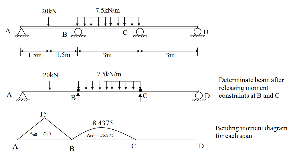 Fig.9.5.
Bending moment diagrams for each span due to external load are obtained using any method discussed in module I.
By inspection we have,
MA = 0 and MD = 0
\[{A_{AB}}={1 \over 2} \times 15 \times 3=22.5\] and \[{x_{AB}}=1.5\]
\[{A_{BC}}={2 \over 3} \times 8.4375 \times 3=16.875\] and \[{x_{CB}}=1.5\]
Now, applying Three-Moment Equation at B,
\[3{M_A} + 2{M_B}\left( {3 + 3} \right) + 3{M_C}=-{{6 \times 22.5 \times 1.5} \over 3} - {{6 \times 16.875 \times 1.5} \over 3}\]
\[\Rightarrow 4{M_B} + {M_C}=-39.375\] (1)
Now, applying Three-Moment Equation at C,
\[3{M_B} + 2{M_C}\left( {3 + 3} \right) + 3{M_D}=-{{6 \times 16.875 \times 1.5} \over 3}\]
\[ \Rightarrow {M_B} + 4{M_C}=-16.875\] (2)
Solving (1) and (2), we have,
\[{M_B}=- 9.375{\rm{kNm}}\] and \[{M_C}=-1.875{\rm{kNm}}\]
After determining the redundant moment, remaining support reaction may be obtained by using static equilibrium equations.
\[\sum {{M_B}}=0 \Rightarrow 3{A_y} - 20 \times 1.5 = {M_B} \Rightarrow 3{A_y} - 20 \times 1.5=-9.375 \Rightarrow {A_y} = 6.875{\rm{kN}}\]
\[\sum {{M_C}}=0 \Rightarrow 6{A_y} + 3{B_y} - 20 \times 4.5 - 7.5 \times 3 \times 1.5 = {M_C}\]
\[\Rightarrow 3{B_y}=-1.875 + 123.75 - 6 \times 6.875 \Rightarrow {B_y} = 26.875{\rm{kN}}\]
\[\sum {{M_C}}=0 \Rightarrow {M_C} - 3{D_y} = {D_y}=- 0.625{\rm{kN}}\]
\[\sum {{F_Y}}=0 \Rightarrow {A_y} + {B_y} + {C_y} + {D_y} = 20 + 7.5 \times 3 \Rightarrow {C_y} = 9.375{\rm{kN}}\]
Suggested Readings
Hbbeler, R. C. (2002). Structural Analysis, Pearson Education (Singapore) Pte. Ltd.,Delhi.
Jain, A.K., Punmia, B.C., Jain, A.K., (2004). Theory of Structures. Twelfth Edition, Laxmi Publications.
Menon, D., (2008), Structural Analysis, Narosa Publishing House Pvt. Ltd., New Delhi.
Hsieh, Y.Y., (1987), Elementry Theory of Structures , Third Ddition, Prentrice Hall.
Last modified: Wednesday, 18 September 2013, 10:26 AM