Site pages
Current course
Participants
General
MODULE 1. Analysis of Statically Determinate Beams
MODULE 2. Analysis of Statically Indeterminate Beams
MODULE 3. Columns and Struts
MODULE 4. Riveted and Welded Connections
MODULE 5. Stability Analysis of Gravity Dams
Keywords
LESSON 20. Approximate analysis of fixed and continuous beams - 1
Sometimes the configuration and complexity of the structures may be such that the exact method of analysis is either not available or unfeasible to apply. In such cases, an approximate methods my be constituted based on some simple and yet reasonable assumptions. In this lesson and the next lesson we will determine approximate solutions for some common types of statically indeterminate structures. .
20.1 Portal Method for Frames Subjected to Lateral Load
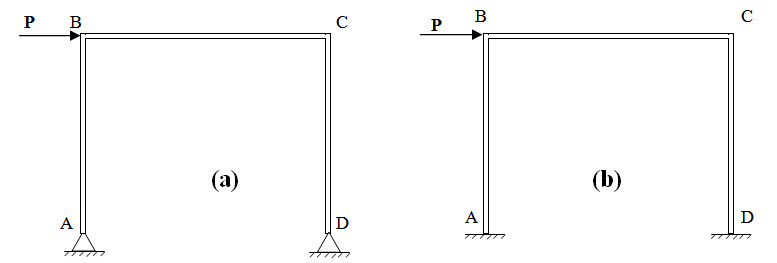
Fig. 20.1.
Consider a portal frame as shown in Fgiure 20.1a. The unknown reaction components are Ax, Ay, Dx and Dy which can not be determined by three equilibrium conditions. Therefore the structure is statically indeterminate with indeterminacy one. Analysis of this structure through the other methods (for statically indterminate structures) shows that . Now while analysing such frame if it is assumed a priori that the horizontal reactions at both legs are same i.e., , the number of unknown reaction components is reduced to three viz. Ay, Dy and H which can be determined through three equations of statics.
Consider another case of the same portal frame but legs are fixed as shwon in Figure 20.2b. The six unknown reaction components are Ax, Ay, MA, Dx, Dy and MD,. Hence the structure is indeterminate with indeterminacy three. In order to have a complete solution of the structure three assumptions must be made. Following are the observations based on analysis of this structure through the other methods (for statically indterminate structures),
-
Horizontal reactions at both legs are same i.e., .
-
Near the centre of each leg bending moment changes its sign (Figure 20.2a) and hence has zero value. These points are called points of inflection.
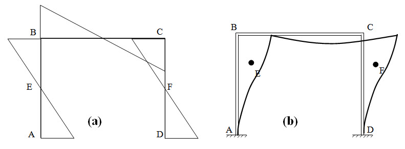
Fig.20.2
Based on the first observation it is assumed \[{A_x}={D_x}\] . This reduces the degree of indeterminacy by one.
Based on the second observation it is assumed that there is a point of inflection at the centre of each leg. This is equivalent to assuming that hinges exist at the centre of each leg i.e, at E and F (Figure 20.2b). Each intermediate hinge gives one additional equation and therefore reduces indeterminacy by one.
Combining above two assumptions, now the degree of indeterminacy of the structure is,
3 – 1 (assumption 1) – 2´ 1(assumption 2) = 0
Therefore the structure now becomes determinate. The above method is illustrated in the following example.
Example 1: Single bay and single storey
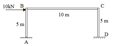
Fig. 20.3.
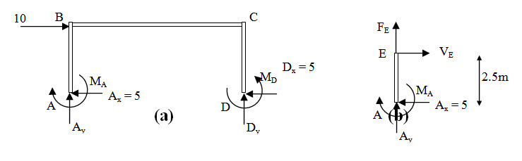
Fig. 20.4.
Assumption 1 gives,
\[{A_x} = {D_x} = 10/2 = 5{\rm{ kN}}\]
According to assumption 2, moment at E is zero,
\[\sum {{M_A}}=0 \Rightarrow 2.5 \times 5 + {M_A}=0 \Rightarrow {M_A}=-12.5{\rm{ kNm}}\] [Figure 20.4b]
Similarly \[{M_D}=12.5{\rm{ kNm}}\]
Taking moment about A,
\[\sum {{M_A}}=0 \Rightarrow {M_A} - {M_D} + 10 \times 5 - 10 \times {D_y} = 0 \Rightarrow - 12.5 - 12.5 + 50 - 10 \times {D_y}= 0\]
\[\Rightarrow {D_y}=2.5{\rm{ kN}}\]
\[\sum {{F_y}}=0 \Rightarrow {A_y} + {D_y}=0 \Rightarrow {A_y}=-2.5{\rm{ kN}}\]
Final solution,
\[{A_x}={D_x}=5{\rm{ kN}}\] ; \[-{A_y} = {D_y}=2.5{\rm{ kN}}\] and \[-{M_A}={M_D}=12.5{\rm{ kNm}}\]
Example 2: Multiple bays and multiple storeys
In practical situations building frames constitute multiple bays and multiple stories as shown in Figure 20.5. Here we will learn how to analyse such frames using portal method.
Assumptions
-
Point of inflection exist at the mid-point of each girder and column.
-
The total horizontal shear at each storey is divided between the columns of that storey such that the interior column carries twice the shear of exterior column.
The last assumption is arrived at by considering each bay as a portal as shown in Figure 20.6. Interior columns are composed of two columns and thus carries twice the shear of exterior column.
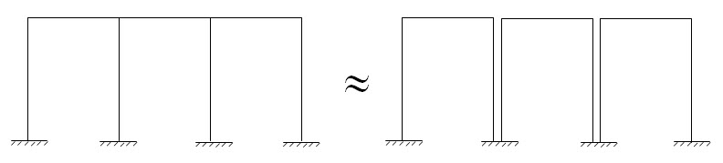
Fig. 20.5.
The portal method is illustrated via the following example.
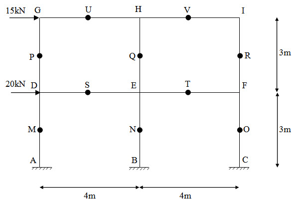 Fig. 20.6.
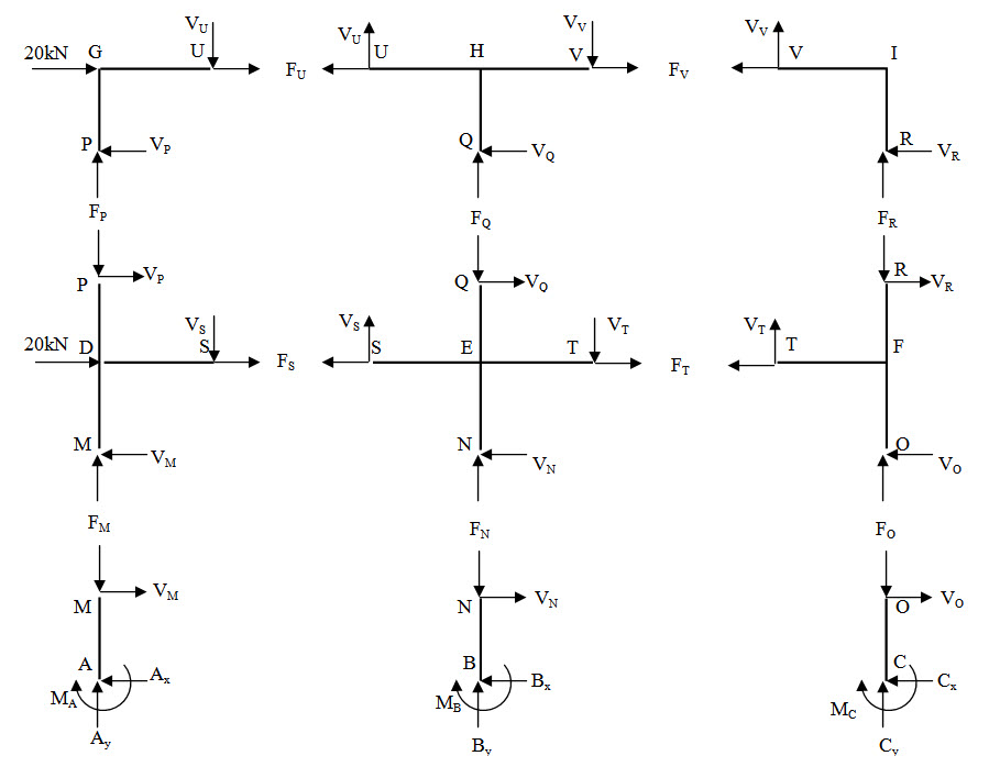
Fig. 20.7
Free body diagrams of different parts of the structures are shown in Fgiure 20.7.
From assumption 2, \[2{A_x}= 2{C_x}={B_x}\] and \[2{V_P}=2{V_R}={V_Q}\]
For first storey, \[{A_x} + {B_x} + {C_x}=20 + 20\] \[\Rightarrow {A_x}=10{\rm{ kN}}\] , \[{B_x}=20{\rm{ kN}}\] and \[{C_x}=10{\rm{ kN}}\]
For second storey, \[{V_A} + {V_C} + {V_B}=20\] \[\Rightarrow {V_P}=5{\rm{ kN}}\] , \[{V_Q}=10{\rm{ kN}}\] and \[{V_R}=5{\rm{ kN}}\]
\[\sum {{M_M}}=0 \Rightarrow {M_A} + 1.5 \times {V_A}=0 \Rightarrow {M_A}=-15{\rm{ kNm}}\]
\[\sum {{M_N}}=0 \Rightarrow {M_A} + 1.5 \times {V_A}=0 \Rightarrow {M_A}=-15{\rm{ kNm}}\]
\[\sum {{M_O}}=0 \Rightarrow {M_A} + 1.5 \times {V_A}=0 \Rightarrow {M_A}=-15{\rm{ kNm}}\]
\[\sum {{M_U}}=0 \Rightarrow 1.5 \times {V_P} + 2 \times {F_P}=0 \Rightarrow {F_P}=-3.75{\rm{ kN}}\]
\[\sum {{M_V}}=0 \Rightarrow 1.5 \times {V_R} - 2 \times {F_R}=0 \Rightarrow {F_R}=3.75{\rm{ kN}}\]
\[{F_P} + {F_Q} + {F_R}=0 \Rightarrow {F_Q}=0\]
\[{A_y}={F_M}={F_P}=-3.75{\rm{ kN}}\]
\[{B_y}={F_N}={F_Q}=0\]
\[{C_y}={F_O}={F_R}=3.75{\rm{ kN}}\]
An illustration of determining unknown support reactions are given above. Similarly by considering free body diagram of different parts as shown in Figure 20.7 and applying equlibrium conditions, member forces can also be determined.
Suggested Readings
Hbbeler, R. C. (2002). Structural Analysis, Pearson Education (Singapore) Pte. Ltd.,Delhi.
Jain, A.K., Punmia, B.C., Jain, A.K., (2004). Theory of Structures. Twelfth Edition, Laxmi Publications.
Menon, D., (2008), Structural Analysis, Narosa Publishing House Pvt. Ltd., New Delhi.
Hsieh, Y.Y., (1987), Elementry Theory of Structures , Third Ddition, Prentrice Hall.
Last modified: Thursday, 19 September 2013, 5:32 AM