Site pages
Current course
Participants
General
MODULE 1. Analysis of Statically Determinate Beams
MODULE 2. Analysis of Statically Indeterminate Beams
MODULE 3. Columns and Struts
MODULE 4. Riveted and Welded Connections
MODULE 5. Stability Analysis of Gravity Dams
Keywords
LESSON 18. Displacement Method: Moment Distribution Method – 4
18.1 Introduction : In this lesson the application of the Moment Distribution Method in frames where joint translations (side sway) are restrained is illustrated via two examples.
18.1.1 Example 1
Draw the bending moment diagram for the follwing frame. EI is constant for all members.
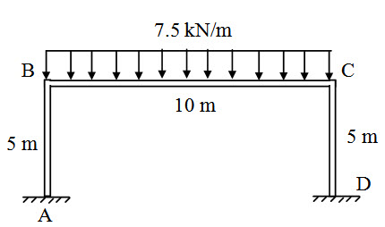
Fig. 18.1.
\[{k_{BA}}={{4E{I_{BA}}} \over {{L_{BA}}}}={{4EI} \over 5}\] , \[{k_{BC}}={{4E{I_{BC}}} \over {{L_{BC}}}}={{2EI} \over 5}\] and \[{k_{CD}}={{4E{I_{CD}}} \over {{L_{CD}}}}={{4EI} \over 5}\]
Distribution factors for BA and BC are,
\[D{F_{BA}}={2 \over 3}\] , \[D{F_{BC}}={1 \over 3}\] , \[D{F_{CB}}={1 \over 3}\] and \[D{F_{CD}}={2 \over 3}\]
End A and D are fixed and therefore no moment will be carrid over to B and C from A and D respectively. Carry over factors for other joints,
\[C_{BA}={1 \over 2}\] , \[C_{BC}={1 \over 2}\] , \[C_{CB}={1 \over 2}\] and \[C_{CD}={1 \over 2}\]
Fixed end moments are,
\[M{}_{FBC}=-{{7.5 \times {{10}^2}} \over {12}}=-62.5{\rm{kNm}}\] ; \[M{}_{FCB}={{7.5 \times {{10}^2}} \over {12}}=62.5{\rm{kNm}}\]
\[M{}_{FAB} = M{}_{FBA} = M{}_{FCD} = M{}_{FDC}=0\] .
Calculations are performed in the following table.
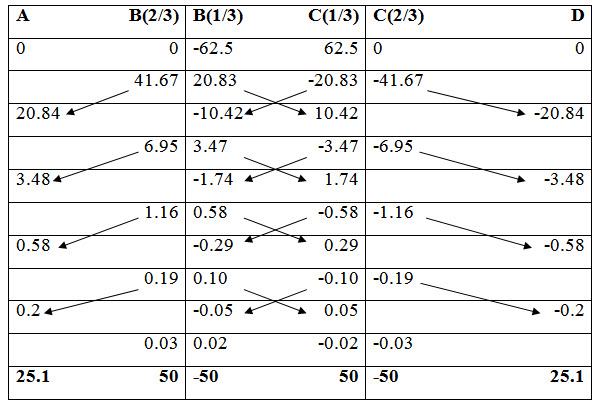

Fig. 18.2. Bending moment diagram (in kNm).
Example 2
Draw the bending moment diagram for the following rigid frame.
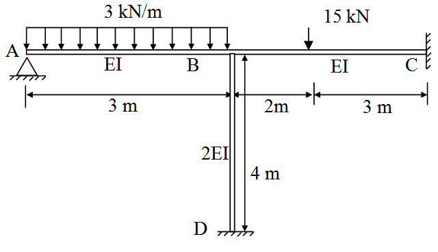 Fig. 18.3.
\[{k_{BA}} = {{3E{I_{BA}}} \over {{L_{BA}}}} = {{3EI} \over 3} = EI\] , \[{k_{BC}} = {{4E{I_{BC}}} \over {{L_{BC}}}} = {{4EI} \over 5}\] and \[{k_{BD}} = {{4E{I_{BC}}} \over {{L_{BC}}}} = {{8EI} \over 4} = 2EI\]
Distribution factors for BA and BC are,
\[D{F_{BA}} = {5 \over {19}}\] , \[D{F_{BC}} = {4 \over {19}}\] and \[D{F_{BD}} = {{10} \over {19}}\]
End C and D are fixed and therefore no moment will be carrid over to B from C and D. Carry over factors for other joints,
\[{C_{AB}} = {1 \over 2}\] , \[{C_{BA}} = {1 \over 2}\] , \[{C_{BC}} = {1 \over 2}\] , \[{C_{BD}} = {1 \over 2}\]
Fixed end moments are,
\[M{}_{FAB}=-{{3 \times {3^2}} \over {12}}=-2.25{\rm{ kNm}}\] ; \[M{}_{FBA} = {{3 \times {3^2}} \over {12}} = 2.25{\rm{ kNm}}\]
\[M{}_{FBC}=-{{15 \times 2 \times {3^2}} \over {{5^2}}}=-10.8{\rm{ kNm}}\] ; \[M{}_{FCB} = {{15 \times 3 \times {2^2}} \over {{5^2}}} = 7.2{\rm{ kNm}}\]
Calculations are performed in the following table.
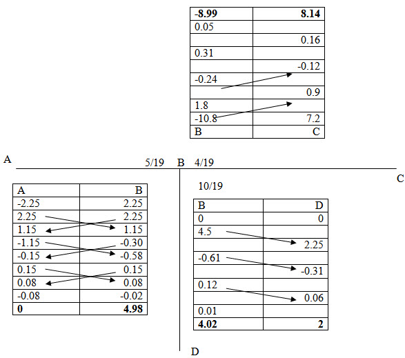
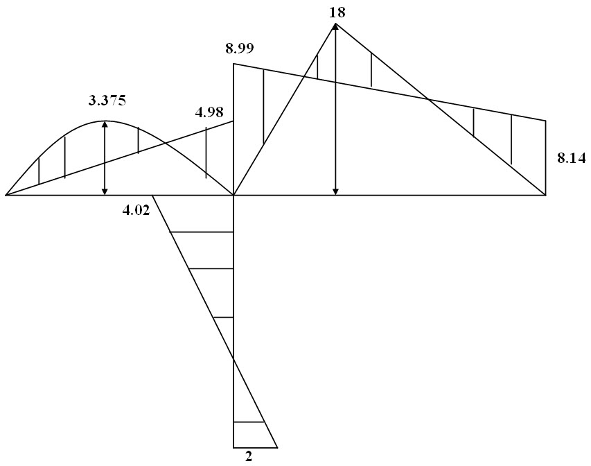
Fig. 18.4. Bending moment diagram.
Suggested Readings
Hbbeler, R. C. (2002). Structural Analysis, Pearson Education (Singapore) Pte. Ltd.,Delhi.
Jain, A.K., Punmia, B.C., Jain, A.K., (2004). Theory of Structures. Twelfth Edition, Laxmi Publications.
Menon, D., (2008), Structural Analysis, Narosa Publishing House Pvt. Ltd., New Delhi.
Hsieh, Y.Y., (1987), Elementry Theory of Structures , Third Ddition, Prentrice Hall.
Last modified: Saturday, 21 September 2013, 4:55 AM