Site pages
Current course
Participants
General
MODULE 1. Analysis of Statically Determinate Beams
MODULE 2. Analysis of Statically Indeterminate Beams
MODULE 3. Columns and Struts
MODULE 4. Riveted and Welded Connections
MODULE 5. Stability Analysis of Gravity Dams
Keywords
LESSON 13. Displacement Method: Slope Deflection Equation – 3
In this lesson we will apply the slope-deflection method for the analysis of rigid frames. Based on the nature of deformation, rigid frames are classified into two categories,
i) Frames without sidesway: lateral translation of joints are restrained
ii) Frames with sidesway: lateral translation of joints are not restrained
Few examples of frames with and without sidesway are depicted in Fig. 13.1.
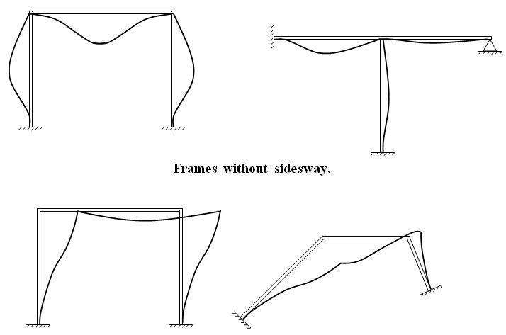
Fig. 13.1. Frames without sidesway.
13.1 Analysis of Frames Without Sidesway
The general procedure for analysis of frames without sidesway is same as for continous beams (lesson 12). This is illustrated in the following two examples.
Example 1
Draw the bending moment diagram for the follwing frame. EI is constant for all members.
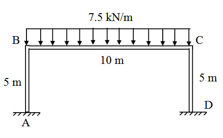 Fig. 13.2.
Step 1: Fixed end Moments
\[M{}_{FAB} =-{{5 \times 4} \over 8}=-2.5{\rm{kNm}}\] ; \[M{}_{FCB} = {{7.5 \times {{10}^2}} \over {12}} = 62.5{\rm{kNm}}\]
\[M{}_{FAB} = M{}_{FBA} = M{}_{FCD} = M{}_{FDC}=0\]
Step 2: Slope-Deflection Equaitons
Since A and D are fixed ends, θA = θD = 0
Since there is no support settlement, δ = 0
For span AB,
\[{M_{AB}} = {M_{FAB}} + {{2EI} \over {{L_{AB}}}}\left( {2{\theta _A} + {\theta _B} - {{3\delta } \over {{L_{AB}}}}} \right) = 0.4EI{\theta _B}\] (13.1)
\[{M_{BA}} = {M_{FBA}} + {{2EI} \over {{L_{AB}}}}\left( {{\theta _A} + 2{\theta _B} - {{3\delta } \over {{L_{AB}}}}} \right) = 0.8EI{\theta _B}\] (13.2)
For span BC,
\[{M_{BC}} = {M_{FBC}} + {{2EI} \over {{L_{BC}}}}\left( {2{\theta _B} + {\theta _C} - {{3\delta } \over {{L_{BC}}}}} \right)=-62.5 + 0.2EI\left( {2{\theta _B} + {\theta _C}} \right)\] (13.3)
\[{M_{CB}} = {M_{FCB}} + {{2EI} \over {{L_{BC}}}}\left( {2{\theta _C} + {\theta _B} - {{3\delta } \over {{L_{BC}}}}} \right) = 62.5 + 0.2EI\left( {{\theta _B} + 2{\theta _C}} \right)\] (13.4)
For span CD,
\[{M_{CD}} = {M_{FCD}} + {{2EI} \over {{L_{CD}}}}\left( {2{\theta _C} + {\theta _D} - {{3\delta } \over {{L_{CD}}}}} \right) = 0.8EI{\theta _C}\] (13.5)
\[{M_{DC}} = {M_{FDC}} + {{2EI} \over {{L_{CD}}}}\left( {{\theta _C} + 2{\theta _D} - {{3\delta } \over {{L_{CD}}}}} \right) = 0.4EI{\theta _C}\] (13.6)
Step 3: Equilibrium Equaitons
At B,
\[{M_{BA}} + {M_{BC}} = 0 \Rightarrow 0.8EI{\theta _B} - 62.5 + 0.2EI\left( {2{\theta _B} + {\theta _C}} \right)=0\]
\[\Rightarrow 1.2EI{\theta _B} + 0.2EI{\theta _C} - 62.5 = 0\] (13.7)
At C,
\[{M_{CB}} + {M_{CD}} = 0 \Rightarrow 62.5 + 0.2EI\left( {{\theta _B} + 2{\theta _C}} \right) + 0.8EI{\theta _C}=0\]
\[\Rightarrow 0.2EI{\theta _B} + 1.2EI{\theta _C} + 62.5 = 0\] (13.8)
Solving equations (7) and (8),
\[{\theta _B} = {{62.5} \over {EI}}\] and \[{\theta _C}=-{{62.5} \over {EI}}\]
Step 4: End Moment calculation
Substituting, θB and θC into equations (1) – (6), we have,
\[{M_{AB}} = 0.4EI{\theta _B} = 25{\rm{ kNm}}\]
\[{M_{BA}} = 0.8EI{\theta _B} = 50{\rm{ kNm}}\]
\[{M_{BC}}=-62.5 + 0.2EI\left( {2{\theta _B} + {\theta _C}} \right) =-50{\rm{ kNm}}\]
\[{M_{CB}} = 62.5 + 0.2EI\left( {{\theta _B} + 2{\theta _C}} \right) = 50{\rm{ kNm}}{M_{CB}} = 62.5 + 0.2EI\left( {{\theta _B} + 2{\theta _C}} \right) = 50{\rm{ kNm}}\]
\[{M_{CD}} = 0.8EI{\theta _C} =-50{\rm{ kNm}}\]
\[{M_{DC}} = 0.4EI{\theta _C} =-25{\rm{ kNm}}\]
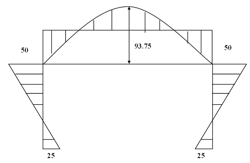
Fig. 13.3. Bending Moment Diagram.
Example 2
Draw the bending moment diagram for the follwing frame. EI is constant for all members.
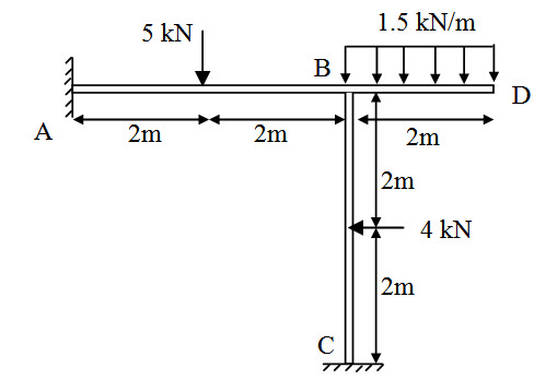
Fig.13.4.
Step 1: Fixed end Moments
\[M{}_{FAB}=-{{5 \times 4} \over 8}=-2.5{\rm{kNm}}\] ; \[M{}_{FBA} = {{5 \times 4} \over 8} = 2.5{\rm{kNm}}\]
\[M{}_{FBC}=-{{4 \times 4} \over 8}=-2{\rm{kNm}}\] ; \[M{}_{FCD}=-{{4 \times 4} \over 8}=-2{\rm{kNm}}\]
Step 2: Slope-Deflection Equaitons
Since A and C are fixed ends, θA = θC = 0
Since there is no support settlement, δ = 0
For span AB,
\[{M_{AB}} = {M_{FAB}} + {{2EI} \over {{L_{AB}}}}\left( {2{\theta _A} + {\theta _B} - {{3\delta } \over {{L_{AB}}}}} \right) =-2.5 + 0.5EI{\theta _B}\] (13.9)
\[{M_{BA}} = {M_{FBA}} + {{2EI} \over {{L_{AB}}}}\left( {{\theta _A} + 2{\theta _B} - {{3\delta } \over {{L_{AB}}}}} \right) = 2.5 + EI{\theta _B}\] (13.10)
For span BC,
\[{M_{BC}} = {M_{FBC}} + {{2EI} \over {{L_{BC}}}}\left( {2{\theta _B} + {\theta _C} - {{3\delta } \over {{L_{BC}}}}} \right) =-2 + EI{\theta _B}\] (13.11)
\[{M_{CB}} = {M_{FCB}} + {{2EI} \over {{L_{BC}}}}\left( {2{\theta _C} + {\theta _B} - {{3\delta } \over {{L_{BC}}}}} \right) = 2 + 0.5EI{\theta _B}\] (13.12)
For span BD,
\[{M_{BD}} =-{{1.5 \times {2^2}} \over 2} = - 3{\rm{ kNm}}\] (13.3)
Step 3: Equilibrium Equaitons
At B,
\[{M_{BA}} + {M_{BC}} + {M_{BD}} = 0 \Rightarrow 2.5 + EI{\theta _B} - 2 + EI{\theta _B} - 3 = 0\]
\[\Rightarrow 2EI{\theta _B} - 19.5 = 0 \Rightarrow {\theta _B} = {{1.25} \over {EI}}\]
Step 4: End Moment calculation
Substituting, θB into equations (9) – (12), we have,
\[{M_{AB}} =-2.5 + 0.5EI{\theta _B} =-1.875{\rm{ kNm}}\]
\[{M_{BA}} = 2.5 + EI{\theta _B} = 3.75{\rm{ kNm}}\]
\[{M_{BC}} =-2 + EI{\theta _B} =-0.75{\rm{kNm}}\]
\[{M_{CB}} = 2 + 0.5EI{\theta _B} = 2.265{\rm{ kNm}}\]
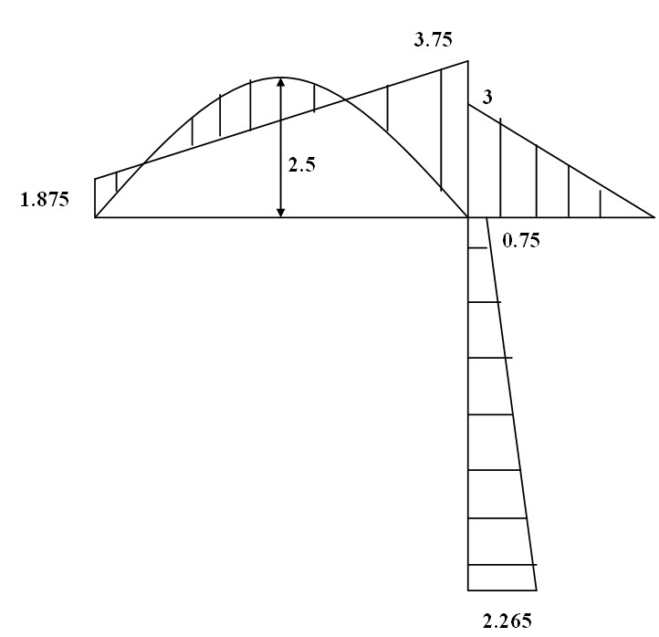
Fig.13.5. Bending Moment Diagram.
Suggested Readings
Hbbeler, R. C. (2002). Structural Analysis, Pearson Education (Singapore) Pte. Ltd.,Delhi.
Jain, A.K., Punmia, B.C., Jain, A.K., (2004). Theory of Structures. Twelfth Edition, Laxmi Publications.
Menon, D., (2008), Structural Analysis, Narosa Publishing House Pvt. Ltd., New Delhi.
Hsieh, Y.Y., (1987), Elementry Theory of Structures , Third Ddition, Prentrice Hall.
Last modified: Wednesday, 18 September 2013, 4:40 AM