Site pages
Current course
Participants
General
MODULE 1. Analysis of Statically Determinate Beams
MODULE 2. Analysis of Statically Indeterminate Beams
MODULE 3. Columns and Struts
MODULE 4. Riveted and Welded Connections
MODULE 5. Stability Analysis of Gravity Dams
Keywords
LESSON 21. Approximate Analysis of Fixed and Continuous Beams – 2
21.1 Introduction : In this lesson we will learn another method, called the Cantilever method for approximate analysis of rigid frames subjected to lateral load. Similar to the Portal method as discussed in the previous lecture, the Cantilever method is also based on few assumptions. These assumptions are as follows,
-
There is a point of inflection at the mid-point of each girder and column.
-
The axial load in each column of a storey is proportional to the horizontal distance of the that column from the centre of gravity of all the column of the storey under consideration.
The above two assumptions give additional equations required for solving unknown reaction components. The method is illustrated via the following examples.
Examples
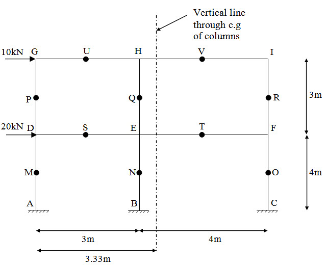
Fig. 21.1.
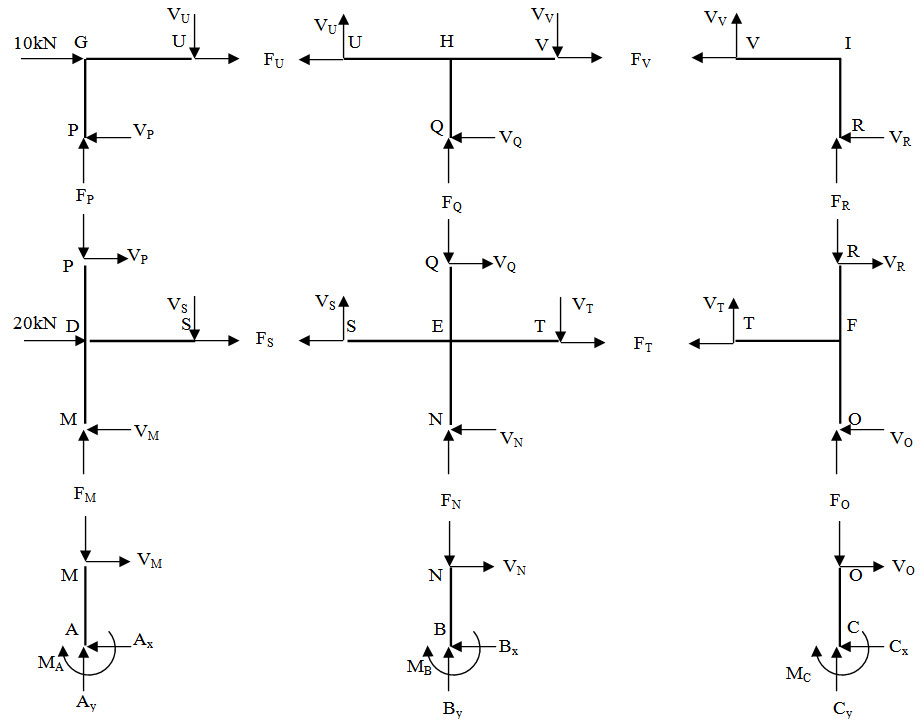
Fig. 21.2.
Free body diagrams of different parts of the structures are shown in Fgiure 20.7. Assuming all columns have the same cross-sectional area, the centre of gravity of the columns for each storey is, \[(3 + 7)/3 = 3.33{\rm{m}}\] from A. Therefore, \[{F_M}\] , \[{F_N}\] and \[{F_O}\] are related as,
\[{F_N} = {{3.33 - 3} \over {3.33}}{F_M} = 0.1{F_M}\] and \[{F_O} = {{3.33 - 7} \over {3.33}}{F_M} =-1.10{F_M}\]
Taking moment about O of all the forces acting on the part above the horizontal plane passing through the points of inflection of the columns of the first storey,
we have,
\[\sum {{M_O}}=0 \Rightarrow 7 \times {F_M} + 4 \times {F_N} + 2 \times 20 + 5 \times 10 = 0\]
\[ \Rightarrow 7 \times {F_M} + 4 \times 0.1{F_M} =-90 \Rightarrow-12.162{\rm{kN}}\]
Hence,
\[{F_N}=0.1{F_M}=-1.216{\rm{kN}}\] and \[{F_O} =-1.10{F_M}=13.378{\rm{kN}}\]
\[{F_P}\] , \[{F_Q}\] and \[{F_R}\] will also follow the similar proportion. Therefore,
\[{F_Q}=0.1{F_P}\] and \[{F_R}=-1.10{F_P}\]
Now taking moment about R, we have,
\[\sum {{M_R}}=0 \Rightarrow 7 \times {F_P} + 4 \times {F_Q} + 2 \times 10 = 0\]
\[\Rightarrow 7 \times {F_P} + 4 \times 0.1 \times {F_P}=-20 \Rightarrow {F_P}=-2.70{\rm{kN}}\]
\[{F_Q} = 0.1{F_P}=-0.27{\rm{kN}}\] and \[{F_R}=-1.10{F_P}=2.97{\rm{kN}}\]
\[\sum {{M_U}}=0 \Rightarrow 1.5 \times {V_P} + 1.5 \times {F_P} = 0 \Rightarrow {V_P} = 2.7{\rm{kN}}\]
\[\sum {{M_V}}=0 \Rightarrow 1.5 \times {V_R}-2 \times {F_R}=0 \Rightarrow {V_R}=3.96{\rm{ kN}}\]
\[{V_P} + {V_Q} + {V_R}=10 \Rightarrow {V_Q}=3.07{\rm{kN}}\]
\[{F_M} - {F_P} - {V_S}=0 \Rightarrow {V_S}=-9.462{\rm{kN}}\]
\[\sum {{M_D}}=1.5 \times {V_P} + 2 \times {V_M} + 1.5 \times {V_S}=0 \Rightarrow {V_M}=5.07{\rm{ kN}}\]
\[{A_x}={V_M}=5.07{\rm{ kN}}\]
\[{A_y}={F_M}=-12.162{\rm{ kN}}\]
\[\sum {{M_M}}=0 \Rightarrow {M_A} + 2 \times {A_x}=0 \Rightarrow {M_A}=-10.14{\rm{ kNm}}\]
An illustration of determining unknown support reactions at A is given above. Similarly by considering free body diagram of different parts as shown in Figure 21.2 and applying equlibrium conditions, other support reactions and member forces can also be determined.
Suggested Readings
Hbbeler, R. C. (2002). Structural Analysis, Pearson Education (Singapore) Pte. Ltd.,Delhi.
Jain, A.K., Punmia, B.C., Jain, A.K., (2004). Theory of Structures. Twelfth Edition, Laxmi Publications.
Menon, D., (2008), Structural Analysis, Narosa Publishing House Pvt. Ltd., New Delhi.
Hsieh, Y.Y., (1987), Elementry Theory of Structures , Third Ddition, Prentrice Hall.
Last modified: Thursday, 19 September 2013, 4:51 AM