Site pages
Current course
Participants
General
MODULE 1. Analysis of Statically Determinate Beams
MODULE 2. Analysis of Statically Indeterminate Beams
MODULE 3. Columns and Struts
MODULE 4. Riveted and Welded Connections
MODULE 5. Stability Analysis of Gravity Dams
Keywords
LESSON 12. Displacement Method: Slope Deflection Equation – 2
12.1 Introduction: In this lesson we will apply the slope -deflection equations, derived in the last lesson, to analyze continuous beams. The general steps are,
Step 1: Treat each span as fixed beam and calculate the fixed end moment. For a ready reference, fixed end moment for a number of common loading cases are summerized in lesson 11.
Step 2: Write slope-deflection equations for each span.
Step 3: Write equilibrium equations for each joint. This will give a set of algebraic equations in terms of unknown rotations. Solve it for the unknown rotations.
Step 4: Substitute the rotations back into the slope-deflection equations and solve for the end moments.
12.1 Example
Calculate the end momens and joint rotations for the continous beam shwon bellow. The beam has constant EI for both the span.
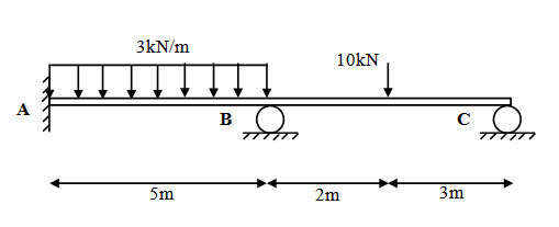
Fig.12.1
Step 1: Fixed end Moments
\[M{}_{FAB}=-{{3 \times {5^2}} \over {12}}=-6.25{\rm{ kNm}}\] ; \[M{}_{FBA} = {{3 \times {5^2}} \over {12}} = 6.25{\rm{ kNm}}\]
\[M{}_{FBC}=-{{10 \times 2 \times {3^2}} \over {{5^2}}}=-7.2{\rm{ kNm}}\] ; \[M{}_{FCB}=-{{10 \times 3 \times {2^2}} \over {{5^2}}} = 4.8{\rm{ kNm}}\]
Step 2: Slope-Deflection Equaitons
For span AB,
\[{M_{AB}} ={M_{FAB}} + {{2EI} \over {{L_{BC}}}}\left( {2{\theta _A} + {\theta _B} - {{3\delta } \over {{L_{BC}}}}} \right)=-6.25{\rm{ }} + {{2EI} \over 5}{\theta _B} =-6.25{\rm{ }} + 0.4EI{\theta _B}\] (1)
\[{M_{BA}} ={M_{FBA}} + {{2EI} \over {{L_{BC}}}}\left( {2{\theta _B} + {\theta _C} - {{3\delta } \over {{L_{BC}}}}} \right) = 6.25 + {{4EI} \over 5}{\theta _B} = 6.25 + 0.8EI{\theta _B}\] (2)
For span BC,
\[{M_{BC}} = {M_{FBC}} + {{2EI} \over {{L_{BC}}}}\left( {2{\theta _B} + {\theta _C} - {{3\delta } \over {{L_{BC}}}}} \right)=-7.2 + {{2EI} \over 5}\left( {2{\theta _B} + {\theta _C}} \right)=-7.2 + 0.4EI\left( {2{\theta _B} + {\theta _C}} \right)\] (3)
\[{M_{CB}} = {M_{FCB}} + {{2EI} \over {{L_{BC}}}}\left( {2{\theta _C} + {\theta _B} - {{3\delta } \over {{L_{BC}}}}} \right) = 4.8 + {{2EI} \over 5}\left( {2{\theta _C} + {\theta _B}} \right) = 4.8 + 0.4EI\left( {2{\theta _C} + {\theta _B}} \right)\] (4)
Step 3: Equilibrium Equaitons
At B,
\[{M_{BA}} + {M_{BC}} = 0 \Rightarrow 6.25 + 0.8EI{\theta _B} - 7.2 + 0.4EI\left( {2{\theta _B} + {\theta _C}} \right)=0\]
\[\Rightarrow 1.6EI{\theta _B} + 0.4EI{\theta _C} - 0.95 = 0\] (5)
At C,
\[{M_{CB}} = 0 \Rightarrow 0.4EI{\theta _B} + 0.8EI{\theta _C} + 4.8 = 0\] (6)
Solving (1) and (2), we have,
\[{\theta _B} = {{2.3929} \over {EI}}\] ; \[{\theta _C}=-{{7.1964} \over {EI}}\]
Step 4: End Moment calculation
Substituting, θB and θC into equations (1) – (4), we have,
\[{M_{AB}}=-6.25{\rm{ }} + 0.4EI{\theta _B} =-5.29\]
\[{M_{BA}} = 6.25 + 0.8EI{\theta _B}=8.16\]
\[{M_{BC}}=-7.2 + 0.4EI\left( {2{\theta _B} + {\theta _C}} \right) =-8.16\]
\[{M_{CB}} = 4.8 + 0.4EI\left( {2{\theta _C} + {\theta _B}} \right)=0\]
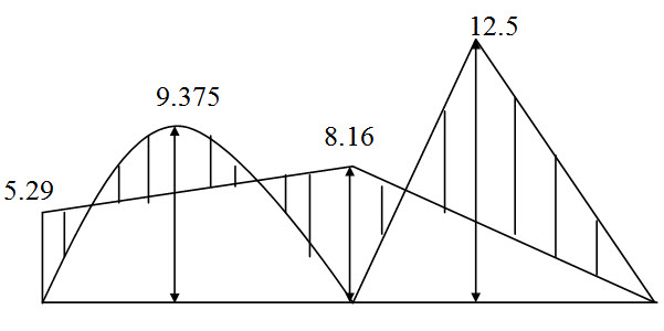
Fig.12.2. Bending moment diagram (kNm).
Suggested Readings
Hbbeler, R. C. (2002). Structural Analysis, Pearson Education (Singapore) Pte. Ltd.,Delhi.
Jain, A.K., Punmia, B.C., Jain, A.K., (2004). Theory of Structures. Twelfth Edition, Laxmi Publications.
Menon, D., (2008), Structural Analysis, Narosa Publishing House Pvt. Ltd., New Delhi.
Hsieh, Y.Y., (1987), Elementry Theory of Structures , Third Ddition, Prentrice Hall.
Last modified: Tuesday, 17 September 2013, 10:53 AM