Site pages
Current course
Participants
General
MODULE 1. Analysis of Statically Determinate Beams
MODULE 2. Analysis of Statically Indeterminate Beams
MODULE 3. Columns and Struts
MODULE 4. Riveted and Welded Connections
MODULE 5. Stability Analysis of Gravity Dams
Keywords
LESSON 11. Displacement Method: Slope Deflection Equation – 1
In the displacement method, unlike the force methods, displacements/rotations at joints are taken as unknowns. A set of algebraic equations in terms of unknown displacements/rotations is obtained by substituting the force-displacement relations into the equilibrium equations. Obtained equations are then solved for the unknown displacements/rotations.
In this lesson and the subsequent lessons we will learn two commonly used displacement method, i) Slope-deflection method, and ii) Moment distribution method.
11.1 Kinematic Unknowns
Since displacements/rotations are the primary unknown, identification of possible displacemnts/rotations at every joint is important. Total number of such unknowns is called kinematic unknowns. For instance, in the shown in Figure 11.1a, joints A and B can only undergo rotation θA and θB respectively and therefore the number of kinematic unknowns is 2. Now if end A is replaced by a fixed support as shown in Figure 11.1b, only possible displacement/roation is qB and therefore the number of kinematic unknowns is reduced to 1. Similarly in Figure 11.1c the kinematic unknowns are θB and δC.
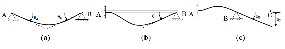
Fig. 11.1.
11.2 Slope-Deflection Method
11.2.1 Sign Convention
For the development and application of Slope-Deflection Method we will use a new sign convention which different from the sign convention discussed in lesson 2.
Moment: At the end of a member clockwise moment is positive.
Transverse displacement: Transverse displacement in upward direction is positive.
Rotation: Rotation in anti-clockwise direction is positive.
The above sign convention is depicted in Figure 11.2.
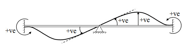
Fig. 11.2.
11.2.2 Basic Concept
Slope-deflection equations are obtained by expressing moment at the end of a member as the superposition of end moment due to external loads on the member assuming ends are restrained and end moments caused by the actual end displacements and rotations. If a structure is composed of several members, which is the case with continuous beam, the above concept is applied to each member seperately. For instance, consider member BC in an arbitrarily loaded continuous beam as shown in Figure 11.3.
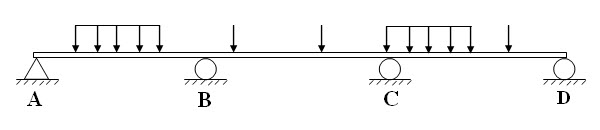
Fig. 11.3.
Let MFBC and MFCB are the end moments due to external loads assuming joint B and C are fixed as shown in Figure 11.4a. δB, θB and δC, θC are the displacement, rotation at joint B and C respectively as shown in Fgiure 11.4b.
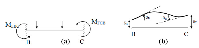
Fig. 11.4.
The end moments at B and C are expressed as:
MBC = MFBC + Moment caused by δB, θB, δC, θC
MCB = MFCB + Moment caused by δB, θB, δC, θC
MFBC/ MFCB are often called as fixed end moment. An illustration of the above concept is discussed in the next sub-section.
11.2.3 Derivation of Slope-Deflection Equations
As mentioned above, in slope-deflection equations, moment at any end is expressed as the sum of fixed end moment and moments due to deflection/rotation.
Fixed end moment
Fixed end moment may be determined by any standard method for solving fixed beam subjected to transverse loading. For ready reference, the fixed end moment for a number of common loading cases are given bellow.
Moment due to rotation at B (= qB)
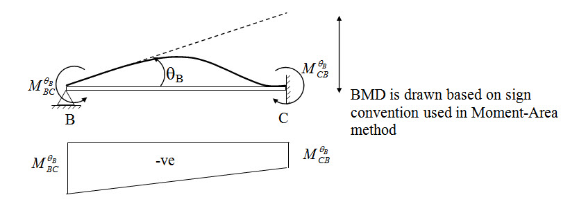
Fig. 11.5.
Let \[M_{BC}^{{\theta _B}}\] and \[M_{CC}^{{\theta _B}}\] are the moment respectively at B and C due to rotation θB at B. Applying Moment-Area method as discussed in Lesson 5, we have,
B. Applying Moment-Area method as discussed in Lesson 5, we have,
\[{\theta _B} = {\rm{Area of M/EI diagram}}\]
\[{\Delta _B} = {\rm{Moment of M/EI diagram about C}}\]
Therefore,
\[{\theta _B} =-{1 \over {2EI}}\left( {M_{BC}^{{\theta _B}} + M_{CB}^{{\theta _B}}} \right) \times {L_{BC}}\] (1)
\[{\Delta _B}={\theta _B} \times {L_{BC}}=-{1 \over {2EI}}\left( {M_{BC}^{{\theta _B}} + M_{CB}^{{\theta _B}}} \right) \times {L_{BC}} \times \left( {{{{L_{BC}}} \over 2} + {{{L_{BC}}} \over 6}{{M_{BC}^{{\theta _B}} - M_{CB}^{{\theta _B}}} \over {M_{BC}^{{\theta _B}} + M_{CB}^{{\theta _B}}}}} \right)\] (2)
\[\Rightarrow {\theta _B} \times {L_{BC}} = {\theta _B} \times {L_{BC}} \times \left( {{1 \over 2} + {1 \over 6}{{M_{BC}^{{\theta _B}} - M_{CB}^{{\theta _B}}} \over {M_{BC}^{{\theta _B}} + M_{CB}^{{\theta _B}}}}} \right)\]
\[\Rightarrow M_{BC}^{{\theta _B}}=-2M_{CB}^{{\theta _B}}\] (2)
From Equation (2) and Equation (1), we have,
\[M_{CB}^{{\theta _B}}={{2EI{\theta _B}} \over {{L_{BC}}}}\] ; and \[M_{BC}^{{\theta _B}}=-{{4EI{\theta _B}} \over {{L_{BC}}}}\]
Moment due to rotation at C (= θC)
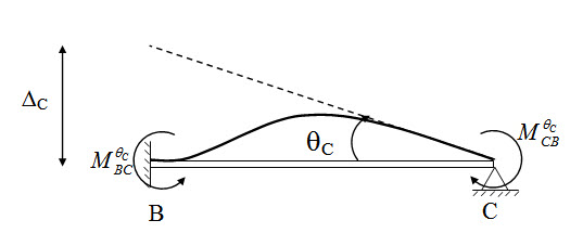
Fig. 11.6.
Following the similar procedure as in the previous case, \[M_{BC}^{{\theta _C}}\] and \[M_{CB}^{{\theta _C}}\] may be obtained as,
\[M_{BC}^{{\theta _B}}=-{{2EI{\theta _B}} \over {{L_{BC}}}}\] and \[M_{CB}^{{\theta _B}}={{4EI{\theta _B}} \over {{L_{BC}}}}\] .
Moment due to δB, δC
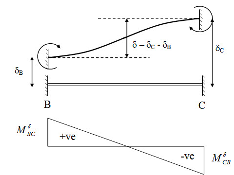
Fig. 11.7.
From the above figure we can write,
Change of slope between tangent at B and C = 0.
=>Area of M/EI diagram = 0
\[\Rightarrow M_{BC}^\delta=M_{CB}^\delta \]
Deviation of point C relative to the tangent drawn to B = Deviation of point Brelative to the tangent drawn to C = δB - δC .
\[\Rightarrow-{1 \over 2}M_{BC}^\delta {{{L_{BC}}} \over 2}{{{L_{BC}}} \over 6} + {1 \over 2}M_{CB}^\delta {{{L_{BC}}} \over 2}\left( {{{{L_{BC}}} \over 2} + {{{L_{BC}}} \over 3}} \right) = \delta \]
\[\Rightarrow-M_{BC}^\delta {{L_{BC}^2} \over {24}} + M_{BC}^\delta {{5L_{BC}^2} \over {24}} = \delta \]
\[\Rightarrow M_{BC}^\delta=-{{6EI\delta } \over {L_{BC}^2}}\]
\[\Rightarrow M_{CB}^\delta=M_{BC}^\delta=-{{6EI\delta } \over {L_{BC}^2}}\]
Finally, the end moments at B and C are obtained by combining the contribution from fixed end moment and joint displacement/rotation as,
\[{M_{BC}}={M_{FBC}} + \left( { - M_{BC}^{{\theta _B}}} \right) + \left( { - M_{BC}^{{\theta _C}}} \right) + M_{BC}^\delta \]
\[{M_{CB}}={M_{FCB}} + M_{CB}^{{\theta _B}} + M_{CB}^{{\theta _C}} + M_{CB}^\delta\]
\[\left[ {\matrix{Moments are added according to the{\rm{}}}\cr{sign convention mentioned in 11.2.1}\cr}\right]\]
Substituting all the relevant terms, we have,
\[{M_{BC}}={M_{FBC}} + {{2EI} \over {{L_{BC}}}}\left( {2{\theta _B} + {\theta _C} - {{3\delta } \over {{L_{BC}}}}} \right)\]
\[{M_{CB}}={M_{FCB}} + {{2EI} \over {{L_{BC}}}}\left( {2{\theta _C} + {\theta _B} - {{3\delta } \over {{L_{BC}}}}} \right)\]
The abover two equations are the Slope-Deflection equation.
Suggested Readings
Hbbeler, R. C. (2002). Structural Analysis, Pearson Education (Singapore) Pte. Ltd.,Delhi.
Jain, A.K., Punmia, B.C., Jain, A.K., (2004). Theory of Structures. Twelfth Edition, Laxmi Publications.
Menon, D., (2008), Structural Analysis, Narosa Publishing House Pvt. Ltd., New Delhi.
Hsieh, Y.Y., (1987), Elementry Theory of Structures , Third Ddition, Prentrice Hall.
Last modified: Tuesday, 17 September 2013, 9:52 AM